Plotting Simulation Results
Saving and Printing the Output in Console Mode
Plotting a diagram is to graphically represent how a dependent variable varies with an independent variable. The independent variable is either distance or time.
- Complete all the steps to run your simulation.
- At the
DICprompt typePOST_PROCESSOR(or justPOST). - Use SET_DIAGRAM_AXIS to specify the variables to plot on the X- and Y-axes of the diagram. One of the axes must be set to either TIME or DISTANCE.
For example, to set the X-axis to plot the distance from the lower boundary of the calculation (rather than from the lower boundary of the current region) and the Y-axis to plot the weight-percent composition of the Si element, at the
POSTprompt type:SET_DIAGRAM_AXIS X DISTANCE GLOBAL
SET_DIAGRAM AXIS Y WEIGHT-PERCENT SI
- You can specify a Z-axis, which is represented as tick marks on the curve in the XY-plane.
- When one of the axes is set to TIME or DISTANCE, the variable automatically becomes the independent variable. If you do not want the independent variable plotted along an axis, use SET_INDEPENDENT_VARIABLE and set it to
TimeorDistance. - Simulation calculations depend on both time and a spatial coordinate; these variables must be fixed during the plotting process. Use SET_PLOT_CONDITION to set the variable to keep fixed. These variables can be set as the fixed plot condition:
Time: The integration time. More than one value can be entered using commas or spaces to separate the values. One graph is plotted for each value.Distance: The distance in the system (from the lower boundary).Interface: At the location of a certain interface between two phases.Intergral: The value of the plot condition is integrated over the phase, region or system volume.
- Use PLOT_DIAGRAM to plot the results. The plot is added as a tab to the Console Results window.
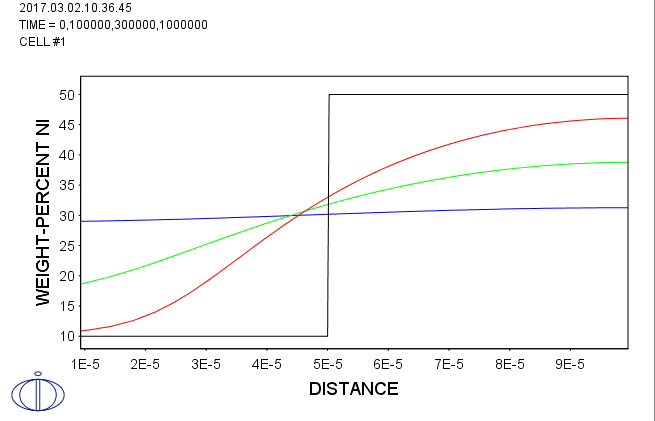
The plot example below is from example exa2a, which is part of the Diffusion Module example collection (see About the Examples in the Thermo‑Calc documentation). Distance is set as the independent variable and the weight-percent of Ni is on the Y-axis. The plot condition is
TIME: the plot shows four graphs, each with the spatial distribution of Ni in the region at the time steps 0, 1e5, 3e5, and 10e5. - To print the plotted graphs direct to a postscript-file, type
Plotand a file name. - In the Plot window, right click the diagram and choose Properties to adjust its appearance and colors.
