Setting up the Single-Phase Simulation
The simulation set-up is performed in the DICTRA_MONITOR module.
goto_module
dictra_monitor
In this example only one global condition is set, temperature. The other global condition that can be set is pressure, but that is rarely done as the default value (1 atm) is set automatically and usually accepted.
SET_CONDITION <GLOBAL OR BOUNDARY>
set_condition global
The SET_CONDITION command is immediately followed by these sub-prompts:
<T OR P>
T
The T is for temperature. Then follows a standard procedure for entering temporally piece-wise functions:
<LOW TIME LIMIT> <FUNCTION> <HIGH TIME LIMIT> <Y/N> <IF Y, THEN NEXT FUNCTION> <...>
0 1400; * N
These prompts start with the low time limit, here zero (0), then the function (here the constant value 1400) closed by a semicolon (;), then the high time limit (here a wildcard * is entered), then a Y or a N depending on whether more functions will be entered (in this case N because only a single function is entered).
The wildcard * used for the upper time limit means that the entered function is valid for the whole simulation. What this means is that a constant temperature equal to 1400 K is used during the whole simulation.
In any simulation at least one region must be defined. This is a named container that designates a certain part of, in this case the whole, domain. The name of a region is arbitrary and specified by you.
ENTER_REGION <NAME OF REGION>
enter_region austenite
The use of regions becomes clearer in the context of so-called moving phase boundary simulations (see About the Moving Phase Boundary Simulation).
A region must contain a numerical grid specified by width and type.
ENTER_GRID_COORDINATES
<NAME OF REGION FOR WHICH GRID IS TO BE ENTERED>
<WIDTH OF REGION>
<TYPE OF GRID>
<NUMBER OF GRID POINTS>
enter_grid_coordinates
austenite
1e-4
auto
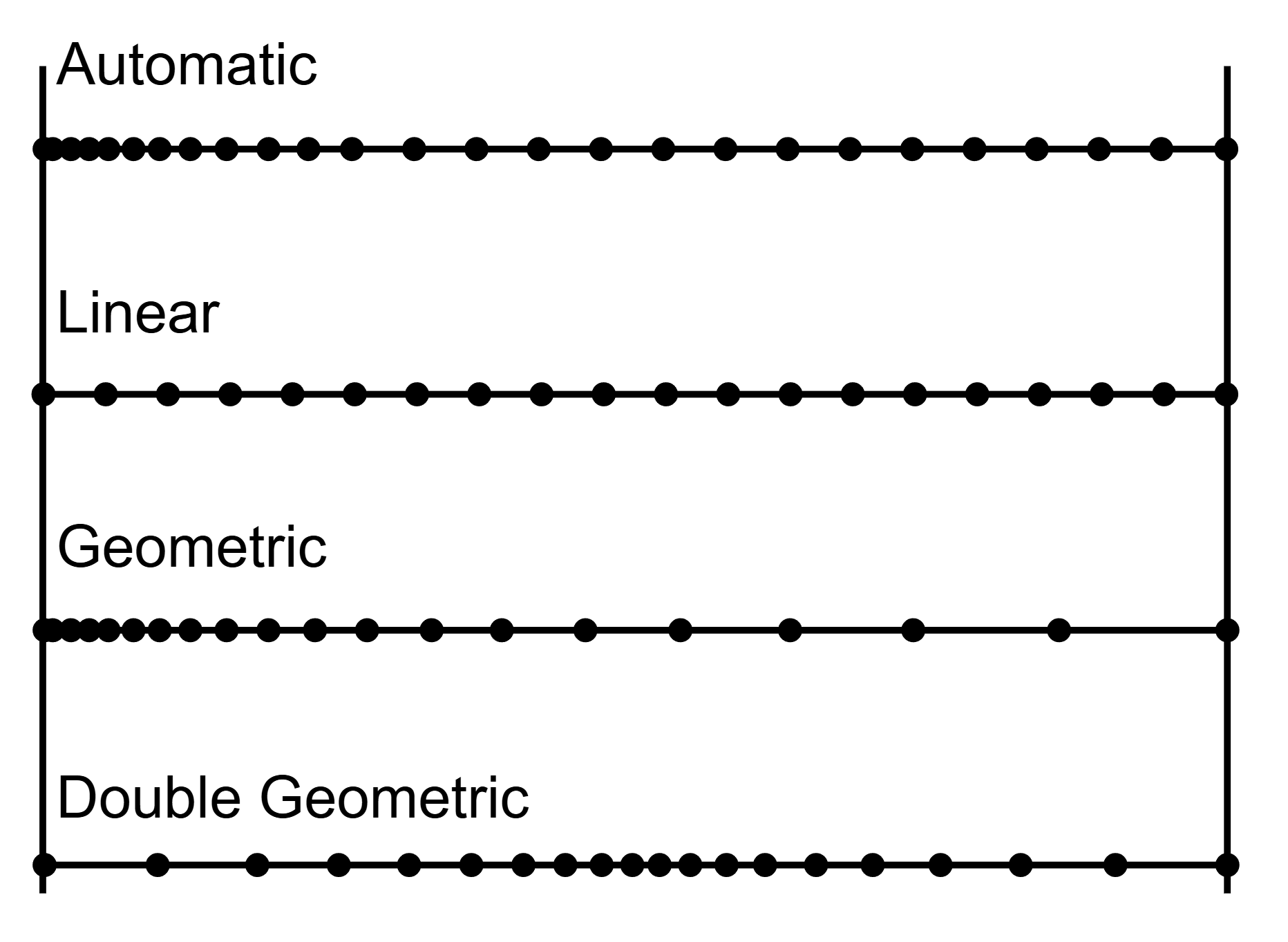
In the entries above, a 10-4 m wide (1e-4), auto. There are many types of grids, and a good choice is the automatic (auto) grid point distribution. An appropriate grid is generated at the start of the simulation where the grid points are automatically distributed according to the entered composition profile and boundary conditions.
These grid types are used in diffusion simulations: automatic, linear, geometric, and double geometric. When you are setting up the simulation, in either Console Mode or Graphical Mode, a region must have a grid defined.
A region must contain one active phase of type matrix. The meaning of active/inactive and phase type is explained in the next examples.
ENTER_PHASE_IN_REGION
<ACTIVE OR INACTIVE>
<NAME OF REGION>
<PHASE TYPE IN REGION>
<PHASE NAME>
enter_phase_in_region
active
austenite
matrix
fcc_a1
In this example only one phase participates, the fcc_a1 phase, and it must therefore be active and of type matrix.
The initial composition profile must be specified for all phases that take part in a simulation. Since there are only two elements, Fe and Ni, in the present simulation the initial composition profile must only be given for one of them.
ENTER_COMPOSITIONS
<REGION NAME>
<PHASE NAME>
<DEPENDENT COMPONENT>
<COMPOSITION TYPE>
<COMPONENT NAME>
<TYPE OF COMPOSITION PROFILE>
<COMPOSITION PROFILE DEPENDENT INPUT>
enter_compositions
austenite
fcc_a1
fe
weight_percent
ni
linear
10
50
In the above entries, Fe is chosen as the dependent component and the initial profile for Ni is a linear variation going from 10 mass-% on the lower/left hand side of the system to 50 mass-% on the upper/right hand side of the system. The composition type can be chosen among a number of different types, e.g. weight percent or mole fraction. There are also many different ways of specifying the composition profile, e.g. an arbitrary position dependent function or reading it for each grid point from file. Here the simplest possible type is used a linear function.
Now you set the simulation time. If not specified the initial time is set to zero.
SET_SIMULATION_TIME
<SIMULATION END TIME>
<AUTOMATIC TIMESTEP CONTROL Y/N>
<MAXIMUM TIMESTEP>
<INITIAL SIZE OF TIMESTEP>
<SMALLEST ALLOWED TIMESTEP>
set_simulation_time
1E5
y
1E4
1E-7
1E-7
Here the simulation time is set to 105 [s] (1E5), the maximum timestep size to 104 (1E4) and the initial and smallest acceptable to 10-7 (both 1E-7). The automatic timestep control should normally always be turned on, which it is by default (you answer Y above).
Now you save the workspace:
SAVE_WORKSPACES <FILENAME> <OVERWITE EXISTING FILE Y/N>
save_workspaces simplest_dictra y
The command name SAVE_WORKSPACES can be misleading. The meaning of this command is roughly set result file. The set-up is saved immediately, but all results during the simulation are also saved to the selected file.
