TC‑Python Thermo-Calc Examples

File name: pyex_T_01_Single-point_equilibrium_looping_and_3d_plotting.py

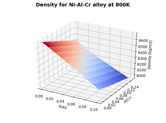
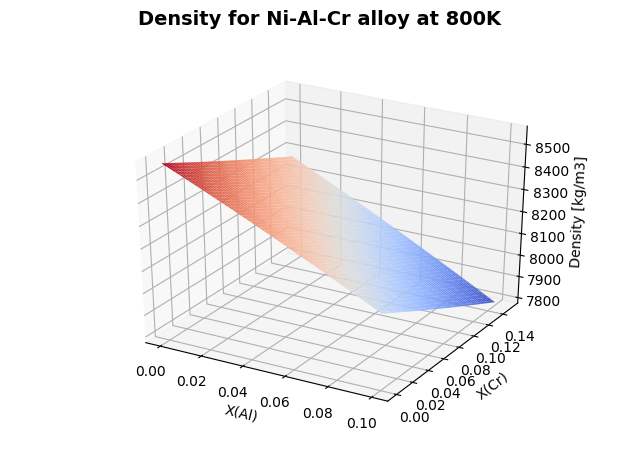
This example shows how you create a single equilibrium calculation from a ternary system, loop it while changing Al and Cr concentration, then calculate density and plot the result as a 3D surface.

Plot showing the density for Ni-Al-Cr alloy at 800 K.

File name: pyex_T_02_Single_equilibrium_solidus_and_liquidus_temperature.py

This example shows how to create a single equilibrium calculation from a ternary system and configure it to calculate the solidus and liquidus temperature using fixed phase conditions for the liquid phase. There can be multiple solutions to a fixed phase condition and it is good practice to perform a regular equilibrium calculation close to where the phase transition is. This example starts with an equilibrium calculation at 1700 K in order to get good start values.

The result from this example is output to the log window.

File name: pyex_T_08_Property_diagram.py

This example shows how to create a property (step) diagram using TC-Python.

The alloy system Fe-Ni is used as an example.

File name: pyex_T_09_Property_diagram_loop_parallel.py

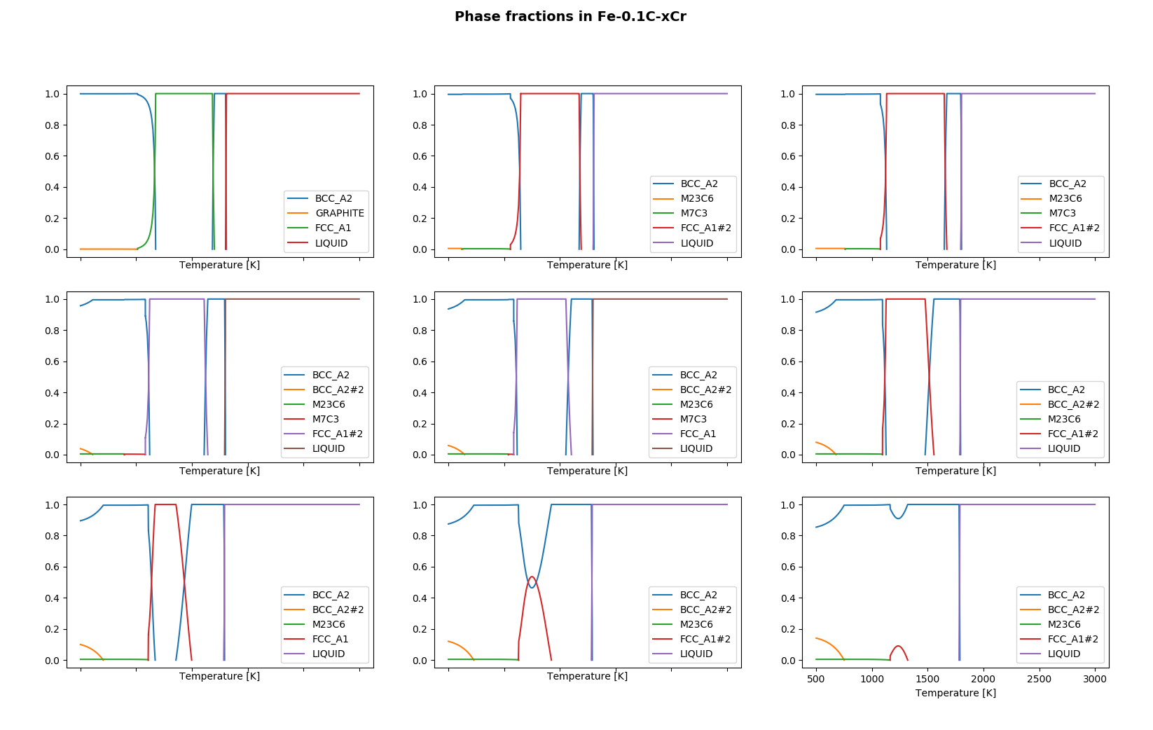
This example shows how to run multiple property (step) diagram calculations in parallel. TC-Python supports parallel computation only by using multi-processing.

The alloy system Fe-C-Cr is used as an example.

Plot results after running multiple property (step) diagrams for an Fe-C-Cr alloy.

File name: pyex_T_10_Property_diagram_alloy_A_to_alloy_B.py

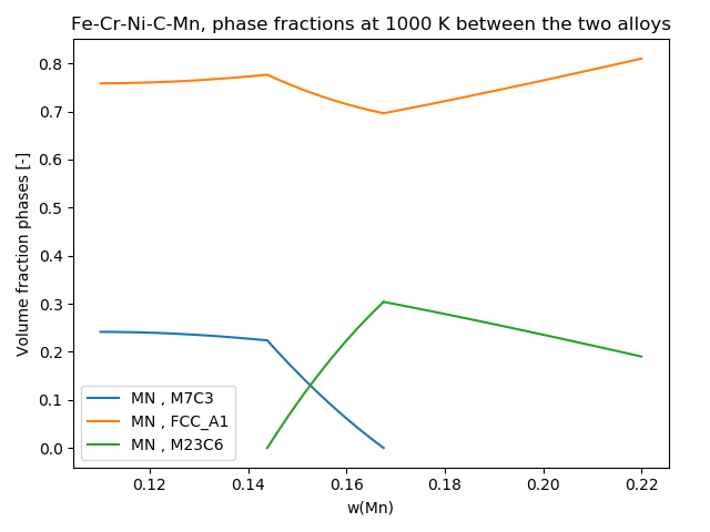
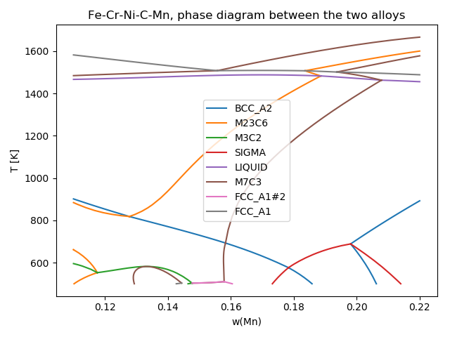
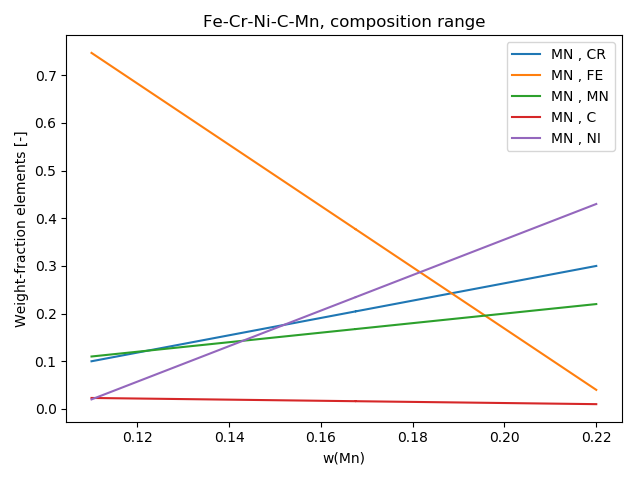
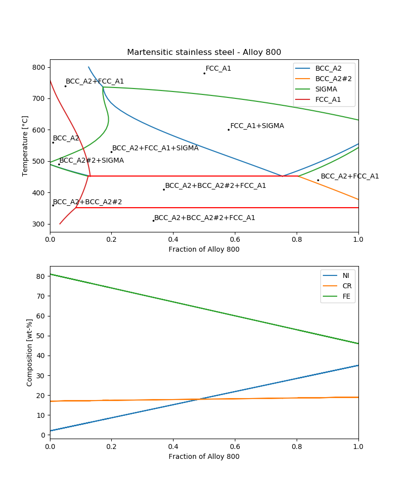
This example shows how to perform step calculations to create property diagrams. The plot results for this example show a section between two materials when moving from one material composition to another. On the left side of the diagram it is one alloy and on the right side it is another alloy.

A property (step) diagram showing how phase fraction varies in the section.

A phase diagram for the same section as the property diagram but with the temperature on the y-axis.

In this plot, the compositions vary linearly along the section.

File name: pyex_T_11_Phase_diagram.py

This example shows how to calculate and plot a phase diagram.

The system Fe-Cr is used as an example.

The phase diagram for Fe-Cr.

File name: pyex_T_12_Phase_diagram_export_to_csv_file.py

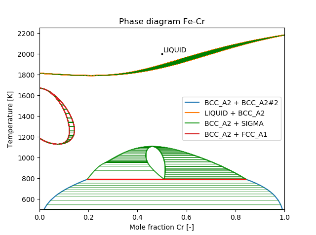
Exports the line data of a phase diagram into a CSV-file that can be imported into other plotting software for creating customized plots for example. It is easy to adapt the code to generate a different format of the CSV-file or to use a completely different output file format.

See CSV Files for the location.

The system Fe-C-Cr is used as an example.

File name: pyex_T_13_Phase_diagram_single_phase_region_shift_Al_Si_Cu.py

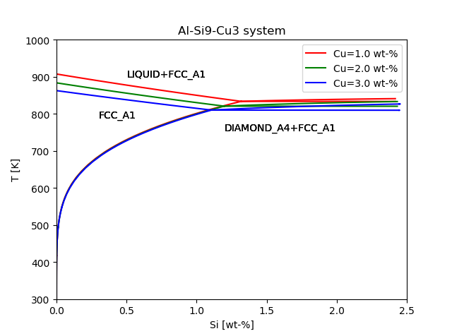
Calculates and plots the single phase FCC_A1 region of Al-Si-Cu alloys and compares them for different Cu-contents.

For simplicity only FCC_A1 and DIAMOND_A4 are enabled as solid phases.

The plot results for the single phase FCC_A1 region of Al-Si-Cu alloys compared to Cu at 1, 2, and 3 wt %.

File name: pyex_T_14_Batch_equilibria.py

This example shows how you create a batch equilibrium calculation from a ternary system, loop it while changing Al and Cr concentration, then calculate the density and plot the result as a 3D surface.

This is almost the same example as pyex_T_01_Single_equilibrium_looping_and_3d_plotting.py, but instead of 100 equilibria it calculates 10000 but only for BCC_A2.

It is much more efficient, since it is using BatchEquilibriumCalculation and not SingleEquilibriumCalculation. BatchEquilibriumCalculation has improved performance when calculating a large number of equilibria when each individual calculations is quick. E.g. when evaluating single phase properties for thousands of compositions.

File name: pyex_T_03_Scheil_mole_fraction_of_solid.py

Shows the basic usage of Scheil calculations in TC‑Python and mixing them with equilibrium calculations.

Plot results showing Solidification of AlSi₁ (top) and mole fraction of all solid phases (bottom).

File name: pyex_T_04_Scheil_composition_distribution_Al_Si_Cu_Mg.py

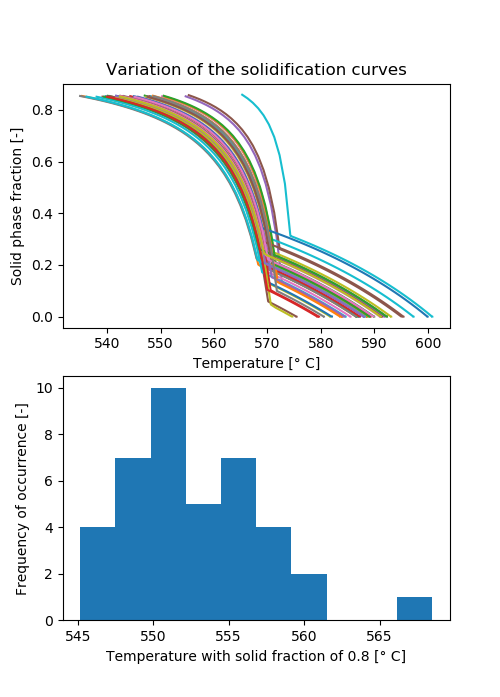
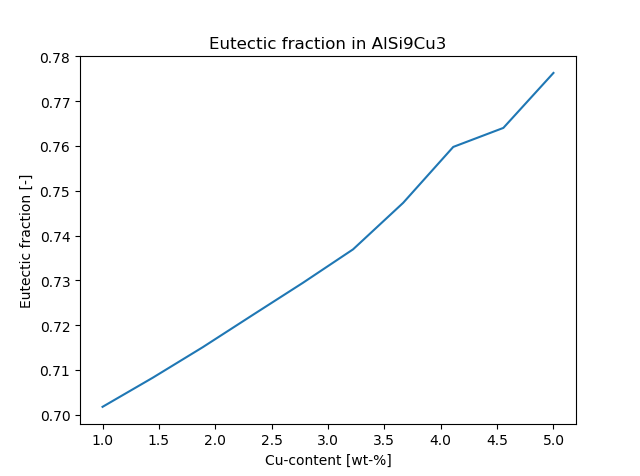
Calculates the variation of the 80% solid temperature using Scheil solidification for random compositions within a specification range.

The alloy system Al-Si-Cu is used as an example.

Plot results showing variation of the solidification curves (top) and how temperature varies by frequency (bottom).

File name: pyex_T_05_Scheil_composition_profiles_Ni_base.py

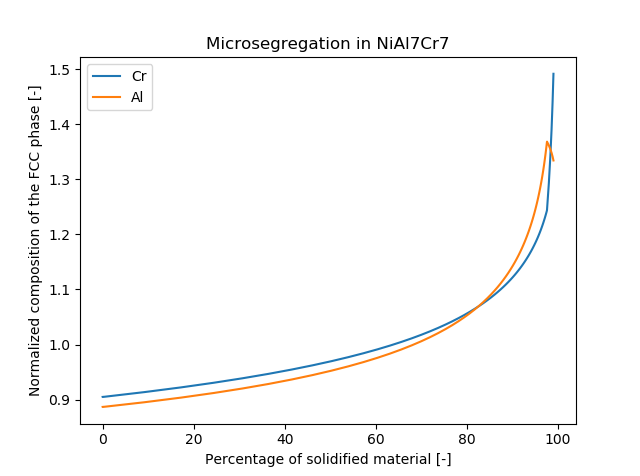
Calculates the microsegregation profile in a solidified Ni-based superalloy using the Scheil-method.

The plot is normalized relative to the nominal composition and shows the composition of the matrix phase (FCC).

A model alloy in the system Ni-Al-Cr is used as an example.

File name: pyex_T_06_Scheil_eutectic_fraction_Al_Si_Cu.py

Calculates the eutectic fraction using Scheil-solidification for varied alloying element content.

The alloy system Al-Si-Cu is used as an example.

Plot result showing Eutectic fraction in Al₅Si₉Cu₃.

File name: pyex_T_07_Scheil_latent_heat_for_solidification_simulations.py

Calculates the characteristic properties of the solidification of a range of alloys using Scheil-solidification and saves the data into a CSV-file (named Al_Si_Cu_scheil_solidification. csv) that can be imported by other software.

See CSV Files for the location.

Such data is typically used as an input into other simulation software, e.g. for casting simulation.

The alloy system Al-Si-Cu is used as an example.

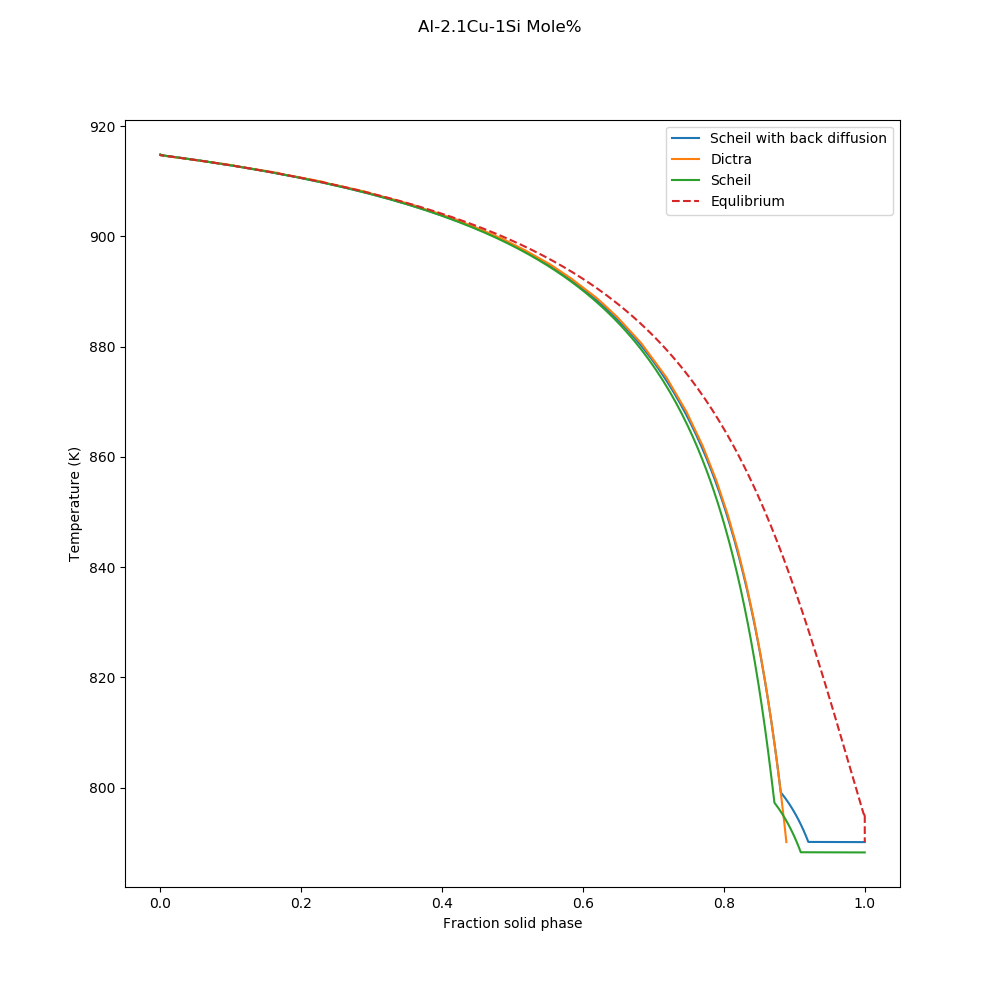
File name: pyex_T_15_Scheil_back_diffusion.py

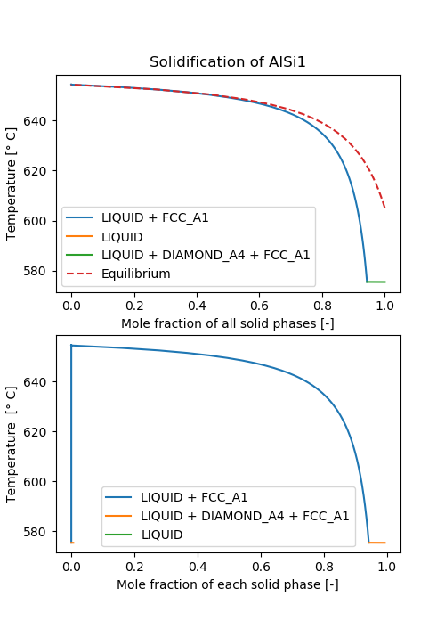
Calculates solidification using Scheil with back diffusion in the primary phase, and compares the result to other calculation types.

Plot result of a Scheil with back diffusion calculation in the primary phase compared to three other calculation types (Diffusion Module (DICTRA), Scheil, and equilibrium).

Calculates the solidification with and without Solute Trapping.

Then compare the solidification in the two cases by plotting temperature vs. mole fraction of solid phase. The alloy system Al-Si-Cu is used as an example.

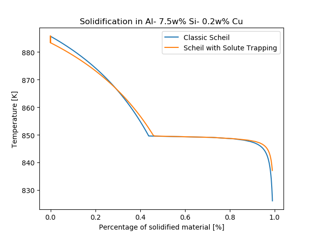
File name: pyex_T_16_Scheil_Solute_Trapping_Al_Si_Cu.py

Graphical Mode example T_13: Scheil Solidification with Solute Trapping.

The effect of Scheil solidification with solute trapping of a Al-7.5Si-0.2Cu alloy compared to a classic Scheil calculation.

Calculates the phases occurring for a material mixture, in this case for a mixture of a martensitic stainless steel with Alloy 800.

This type of calculation is for example useful for understanding effects when welding dissimilar materials - without the need to perform diffusion calculations.

File name: pyex_T_17_Material_to_Material_single_fraction_of_B.py

The result from this example is output to the log window.

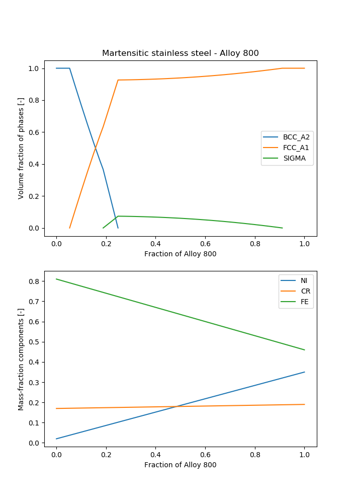
Calculates the phases occurring during a gradual transition between two materials, in this case from a martensitic stainless steel to Alloy 800.

This type of calculation is for example useful for understanding effects when welding dissimilar materials - without the need to perform diffusion calculations.

File name: pyex_T_18_Material_to_Material_step_along_fraction_of_B.py

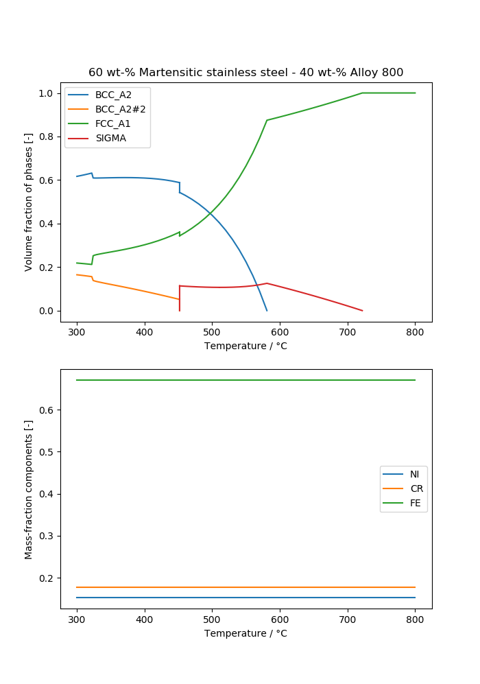
Calculates the phases occurring for a material mixture with varying temperature, in this case for a mixture of a martensitic stainless steel with Alloy 800.

This type of calculation is for example useful for understanding effects when welding dissimilar materials - without the need to perform diffusion calculations.

File name: pyex_T_19_Material_to_Material_step_along_temperature.py

Calculates a "phase diagram" for a material mixture, in this case for a mixture of a martensitic stainless steel with Alloy 800.

This type of calculation is for example useful for understanding effects when welding dissimilar materials - without the need to perform diffusion calculations.

File name: pyex_T_20_Material_to_Material_phase_diagram.py