TC‑Python Diffusion Examples

File name: pyex_D_01_Diffusion_Single_Phase.py

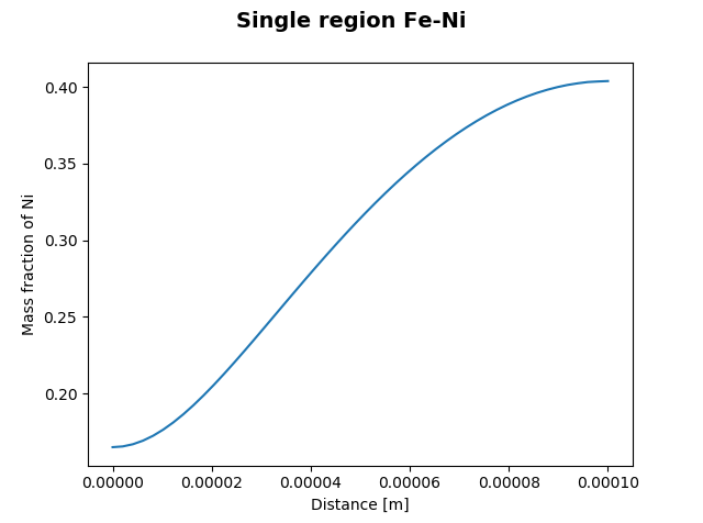
This example simulates diffusion within a single phase austenitic region of an Fe-Ni alloy. The initial condition is a linear gradient from 10 wt-% - 50 wt-% Ni at 1400 K.

The example uses a minimum number of required settings. Default values are used for any unspecified settings.

Also see the Graphical Mode example that this is based on: D_01: Homogenization of a Binary Fe-Ni Alloy.

Single phase austenitic region of an Fe-Ni alloy.

File name: pyex_D_02_Diffusion_Moving_Boundary.py

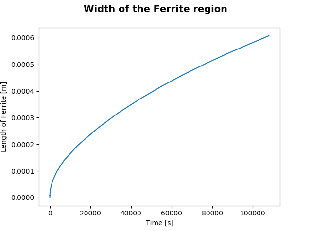
This example simulates diffusion including a moving boundary between a ferrite and austenite region in an Fe-C steel. Initially the C-concentration is constant in each region, with a step at the boundary. All units are in wt-%.

The example uses a minimum number of required settings. Default values are used for any unspecified settings.

Also see the Graphical Mode example that this is based on: D_02: Ferrite(bcc)/Austenite(fcc) Transformation in a Binary Fe-C Alloy.

Plot result showing the width of a ferrite region for an Fe-C steel.

File name: pyex_D_03_Diffusion_Multiphase.py

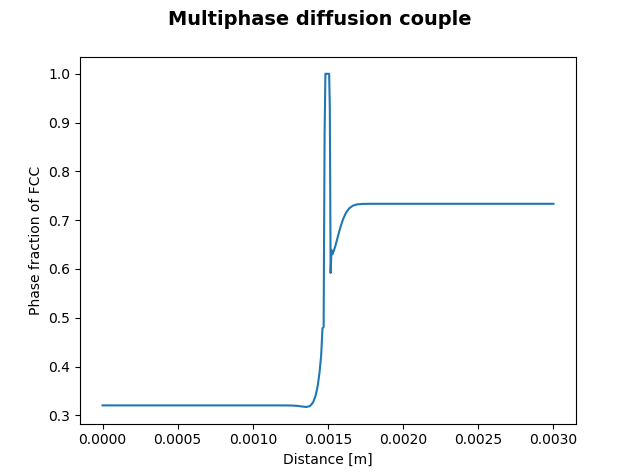
This example simulates diffusion in a single region having multiple phases. Initially a step concentration profile is defined within the single region. Due to the multiple phases, the default AutomaticSolver uses the homogenization mode.

The example uses a minimum number of required settings. Default values are used for any unspecified settings.

Also see the Graphical Mode example that this is based on: D_03: Evolution of an Fe-Cr-Ni Diffusion Couple.

Plot result of diffusion in a single region having multiple phases.

File name: pyex_D_04_Diffusion_Fe-C_Moving_Boundary_Austenite_to_Ferrite.py

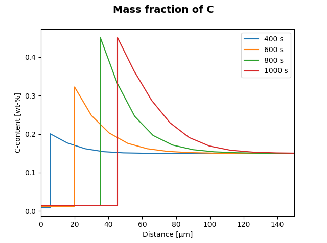
This example simulates a moving boundary problem that is initially a one-phase austenite region. Due to the available driving force, a new ferrite region is starting to grow at the left interface of the austenite region.

Initially a constant concentration profile is defined within the single-phase region.

The example uses a minimum number of required settings. Default values are used for any unspecified settings.

Also see the Graphical Mode example that this is based on: D_04: Fe-C Moving Boundary - Austenite to Ferrite.

Plot result showing the mass fraction of C.

File name: pyex_D_05_Diffusion_Fe_Ni_Cr_Moving_Boundary_Diffusion_Couple.py

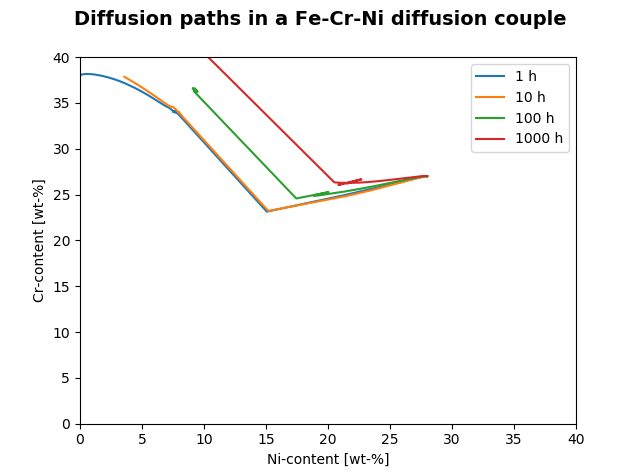
This example simulates the diffusion paths in a moving boundary problem between two multiphase regions. Due to the multiple phases, the default AutomaticSolver uses the homogenization mode.

Initially there is a concentration profile with a step between the regions.

The example uses a minimum number of required settings. Default values are used for any unspecified settings.

Also see the Graphical Mode example that this is based on: D_05: γ/α/γ Diffusion Couple of Fe-Ni-Cr alloys.

Plot result showing diffusion paths in an Fe-Cr-Ni diffusion couple.

File name: pyex_D_06_Deriving_Diffusion_Coefficients_From_Experiment.py

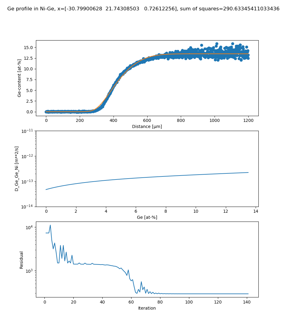
This example demonstrates the direct optimization of mobility database parameters by fitting to experimentally measured composition profiles. A manual determination of the interdiffusion coefficients (for example using the Boltzmann-Matano method) is not required. Additionally, no derivatives of the experimental curve is required as this is difficult for scattered data.

This example takes several minutes to calculate. The results are updated continually. The plot examples shown are the final iterations.

References

The example uses data from:

[2010Liu] Y. Q. Liu, D. J. Ma, and Y. Du, “Thermodynamic modeling of the germanium–nickel system,” J. Alloys Compd., vol. 491, no. 1–2, pp. 63–71, Feb. 2010.

[2011Ret] R. Rettig, S. Steuer, and R. F. Singer, “Diffusion of Germanium in Binary and Multicomponent Nickel Alloys,” J. Phase Equilibria Diffus., vol. 32, no. 3, pp. 198–205, Jun. 2011.

File name: pyex_D_07_Homogenization_Of_Scheil_Profile.py

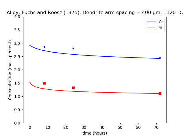
This example models the homogenization of a cast Ni-Cr steel and compares predictions with the experimental data collated by Fuchs and Roósz [1975Fuc].

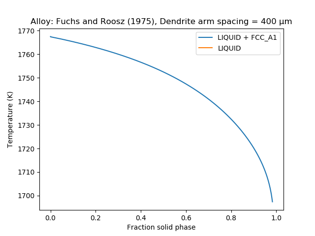
As a first step, the microsegregation after solidification is simulated using a Scheil-calculation, then as a second step the homogenization is simulated using a diffusion simulation.

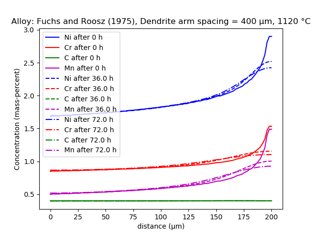
The conditions studied have a dendritic half spacing of 200 µm and are heat treated at 1120 °C.

The data has been de-normalized to allow comparison using weight percent composition values. The composition of the steel is 0.4C, 0.65Mn, 0.35Si, 0.015S, 0.01P, 1.9Ni, 0.95Cr and 0.3 Mo (wt.%). The diffusion of Cr and Ni are modelled using a simplified chemistry of 0.4C, 0.65Mn, 1.9Ni, and 0.95Cr using the FEDEMO thermodynamic and MFEDEMO mobility databases.

Also see the Graphical Mode example that this is based on: D_10: Iron (Fe) Homogenization in Scheil.

Reference

[1975Fuc] E. G. Fuchs, A. Roósz, Homogenization of Iron-Base Cast Alloys. Met. Sci. 9, 111–118 (1975).

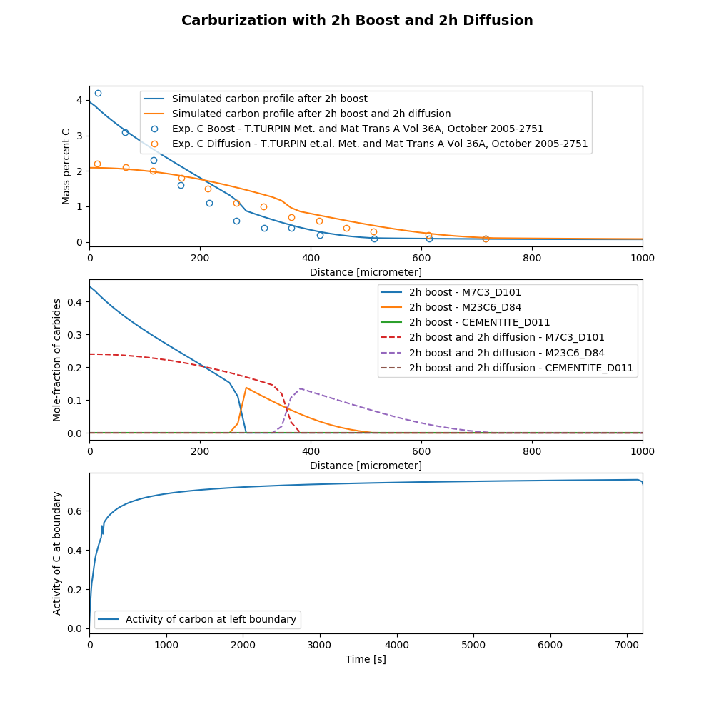
Carburization of an alloy in a two-step procedure with different boundary conditions in each step.

This example requires licenses for TCS Steel and Fe-alloys Database (TCFE) and TCS Steels/Fe-Alloys Mobility Database (MOBFE).

As a first step, the carburization is simulated using a activity-flux boundary condition, then as a second step the homogenization is simulated using a diffusion simulation with closed boundaries.

File name: pyex_D_08_Diffusion_Carburization_Multiphase_Boost_And_Diffusion.py

Reference

Experimental data from:

[2005Tur] T. Turpin, J. Dulcy, and M. Gantois, “Carbon diffusion and phase transformations during gas carburizing of high-alloyed stainless steels: Experimental study and theoretical modeling,” Metall. Mater. Trans. A, vol. 36, no. 10, pp. 2751–2760, Oct. 2005.