About the Uncertainty Calculations
The Uncertainty calculation in Thermo‑Calc uses the values (the mean) entered for quantities under the Condition Definitions section as the starting point to estimate, within a certain probability, the true variation of the quantity. Uncertainty calculations are available with the Property Model Calculator and the Process Metallurgy Calculator.
An example of a Gaussian distribution is shown next. The example uses the Phase Transition Property Model Settings and an Uncertainty Calculation Type to describe how the sampling of data is performed. The example PM_G_01: Phase Transition predicts the transition temperature to the unwanted brittle Sigma phase and shows how the temperature is influenced by changes to a steel alloy’s composition.
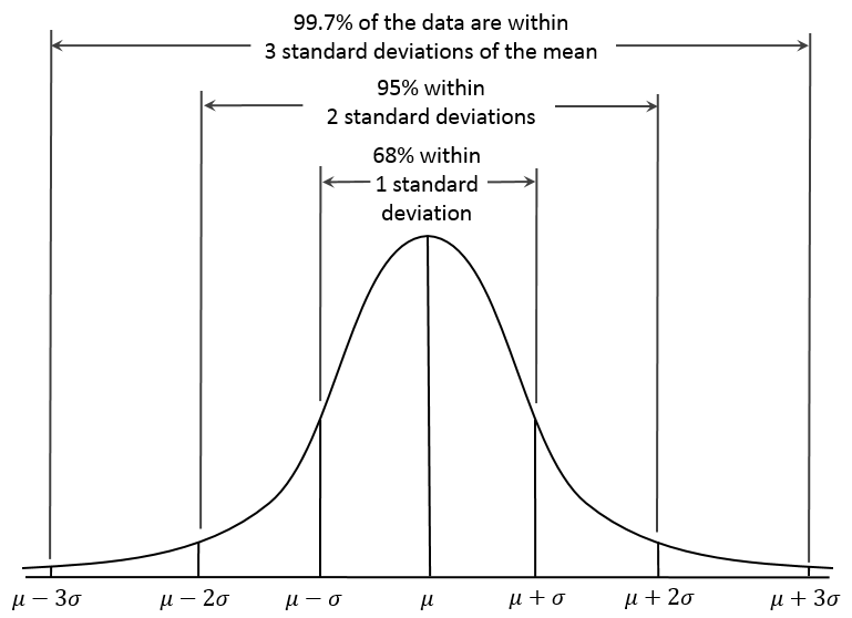
As long as the number of events (the sample size) is very large, then the Gaussian distribution function can be used to describe physical events. A Gaussian distribution is assumed to describe how each quantity varies in an uncertainty calculation, as shown next.
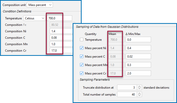
In Thermo‑Calc, the mean of the quantity’s distribution is defined in the Condition Definitions section. The Mean is then used in the Sampling of Data from Gaussian Distributions section as the starting point for how much you want to deviate from this value.
The mean defined under Condition Definitions is used during the sampling.
The values entered in the Δ Min/Max fields are the resulting width of the distribution corresponding to the 95% confidence interval (approximately μ ± 2σ) shown in Gaussian distribution, the 3-sigma rule.This confidence interval means that approximately 95% of the sampled values fall within these limits, as shown next.
The default value for truncating the distribution is set at 3 standard deviations in the Sampling Parameters section. This is also where you set the Total number of samples. The default is 200. In order to maintain a Gaussian distribution for the varied quantities, this number should not be too low.
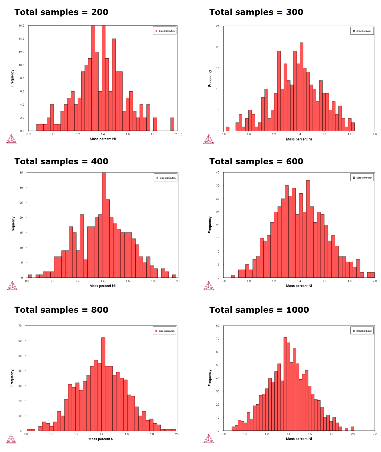
You can experiment by varying the conditions and the number of samples to see the distribution results smooth out as is to be expected based on the Central Limit Theorem, as shown in the histogram plot. You can also plot the results as a normal probability.
This series of histogram plots shows the uncertainty calculations sampling data from Gaussian distributions. On the Plot Renderer the variable is set to measure the Composition of Ni. It compares the Ni composition where the total sample size is increased. In the example, the initial sample size uses the default, 200, and then the sample size is increased to 300, 400, 600, 800, and 1000, showing how the plot follows the Gauss distribution.
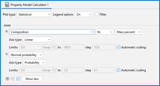
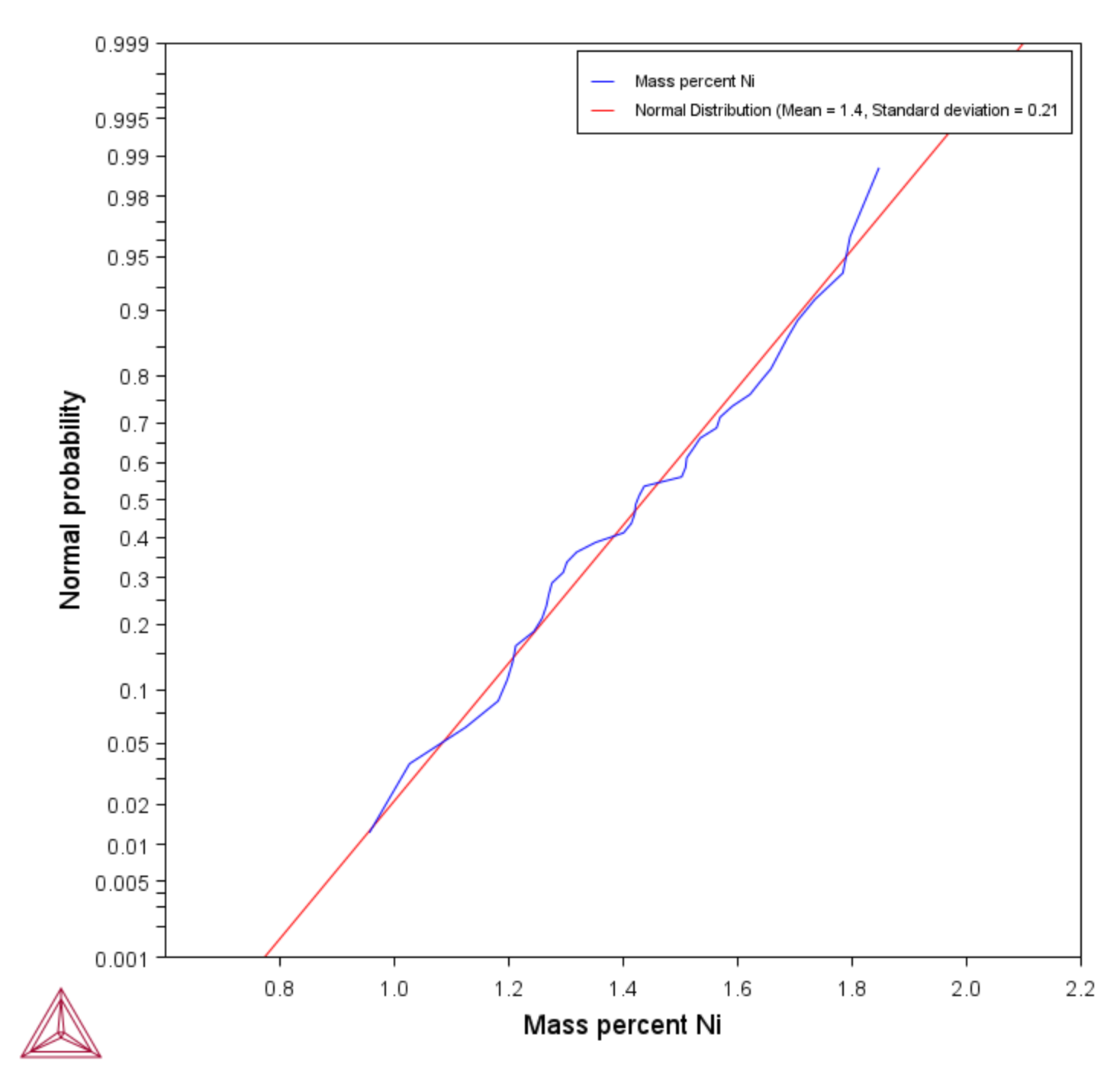
You can also plot the results as a Normal probability. Continuing with this example, for the Property Model Calculator the X variable is plotted as Composition and the Y variable is plotted as the Normal probability.
This is a normal probability plot example of the uncertainty calculations sampling data from Gaussian distributions. It compares the relaxed condition where the total sample size is 200. The sampled data (blue line) closely follows the ideal normal distribution (red line). Deviations are naturally larger at the tails (≈1%Ni and ≈2%Ni) since the number of samples are fewer there compared to the center of the distribution.
