Table Renderer: Configuration Settings

To save all the data in a table as a Character separated (.csv), Hyper Text Markup (.html), or Excel (.xls), in the Configuration window click Save Table or in the Visualizations window right-click in the table and select Save As.

To copy the data from a single cell of a table to the clipboard, right-click the cell and select Copy. To copy the whole table to the clipboard, select Copy all.

The data saved is what is shown in the Table Renderer tab on the Visualizations window. If data is calculated (and not displayed) it is not saved.

The table results can be presented in ordinary decimal number format or with normalized scientific notion. Choose Scientific or Decimal to increase or decrease the number of Decimal digits used in the table. The default is 5 digits. The Number format defaults to Auto to use the most appropriate format based on the tabulated data.

The defaults for these settings can be changed globally.

To open the Options window:

• Windows: Select Tools → Options.
• Mac: Select Thermo-Calc <version> → Preferences or Settings or press <⌘> on the keyboard.

then click the Activities tab and the Tabulation node in the tree.

The quantities are sometimes grouped into categories on the Plot Renderer or Table Renderer. Availability of the list and the variables themselves, is based on several factors, including the database selected, the Calculator used, and the type of calculation being performed. Other differences are based on the Plot type selected, e.g. what you see on the Configuration window changes if you use Flexible Mode or Grouped Mode. Other plot types do not group the quantities and each Calculator handles the information differently.

When working on a Plot Renderer (e.g. associated to the Axes X, Y, and Z) or Table Renderer (associated to Columns), there is sometimes the option to choose a quantity group from a list. When applicable, these are the categories:

• All variables
• System variables
• Phase equilibria
• Physical properties
• Kinetic properties
• Elastic properties

After selecting the group, you next choose from the available variables and continue to define each based on the additional settings specifically available, i.e. select a unit or a phase, and many other options that are only displayed when relevant.

Quantities Groups Available for Plots and Tables

For the Process Metallurgy Calculator there are additional settings available.

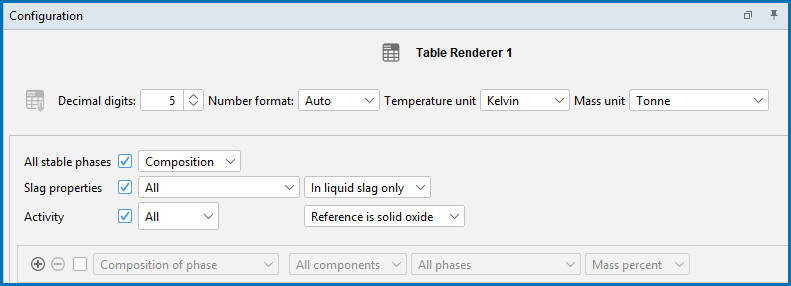
PMET_01: Basic Oxygen Furnace (BOF). Using version 01b, a Table Renderer is added and on the Process Metallurgy Calculator, changed the Calculation Type to Single.

• Choose a Temperature unit: Kelvin, Celsius or Fahrenheit.
• Choose a Mass unit: Tonne, Kilogram, Gram, or Pound.
• Select the All stable phases checkbox and choose Composition or Condensed from the list.
• Select the Slag properties checkbox and choose the associated quantity from the next drop-down list: All, B2, B3, B4, Bas2, Bells ratio, Ls, or Log10 (Sulphur capacity).
• Also choose In liquid slag only, In solid slag only, or In all slag.

  Details, including references and equations, are described in Process Metallurgy Slag Properties.

• Select the Activity checkbox then from the first list choose a component (or keep the default All). Then from the second list select Reference solid oxide or Reference liquid slag.

  The activity is always given relative to a phase. The liquid slag is always the IONIQ_LIQ phase. The composition set of ION_LIQ depends on the calculation and the slag always contains a high amount of oxygen. The reference phase for the solid oxides depends on the components and it is always listed in the table.

When you use a Precipitation Calculator and choose Yield strength as an Axis variable, there are additional settings available.

If you choose Yield strength as an Axis variable, you can further define the model. Click to expand the drop down list to the right of the Axis variable, then select any or all of the checkboxes listed below to plot the respective contributing elements to the yield strength.

Click Configuration Panel toggle between the settings options and to further fine-tune the model. These options are described for the Yield Strength Property Model: Simplified Mode Settings and Yield Strength Property Model: Advanced Mode Settings. The greyed out sections (e.g. the Matrix, Precipitate phases, and Grain size) are defined on the Precipitation Calculator and cannot be changed.

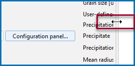
To see these settings after clicking Configuration Panel, you need to expand the Plot Renderer Configuration window to the right. Either detach the window to resize, or hover with the mouse until you see the double arrow, then click and drag to expand the window.

• Total yield strength
• Intrinsic strength
• Solid solution strengthening
• Solid solution strengthening FCC
• Solid solution strengthening BCC
• Solid solution strengthening HCP
• Grain boundary strengthening
• Total precipitation strengthening
• Precipitation strengthening per phase
• Constant strength addition

The P_01: Isothermal Precipitation of Al3Sc example demonstrates the use of this Yield Strength Model.

Yield Strength Property Model: Simplified Mode Settings

When certain axis variables are selected on the Plot Renderer or Table Renderer that is a successor to the Precipitation Calculator, the Separate multimodal PSD and 3D > 2D checkboxes are available for the Precipitation Module (TC-PRISMA).

Another requirement is that the Precipitate Phase Morphology is set to Sphere on the Precipitation Calculator.

See the specialized section for the Plot Renderer for details.

Precipitation Calculator Plot Renderer