PM_Fe_04: Critical Temperatures
The example uses the Property Model Calculator and the Critical Transformation Temperatures Model to calculate the distribution of the typical phase transition temperatures for a low alloy steel (Fe-0.3Cr-1.0Mn-0.3Mn-0.18C) when the composition is varied within the specification for the alloy.
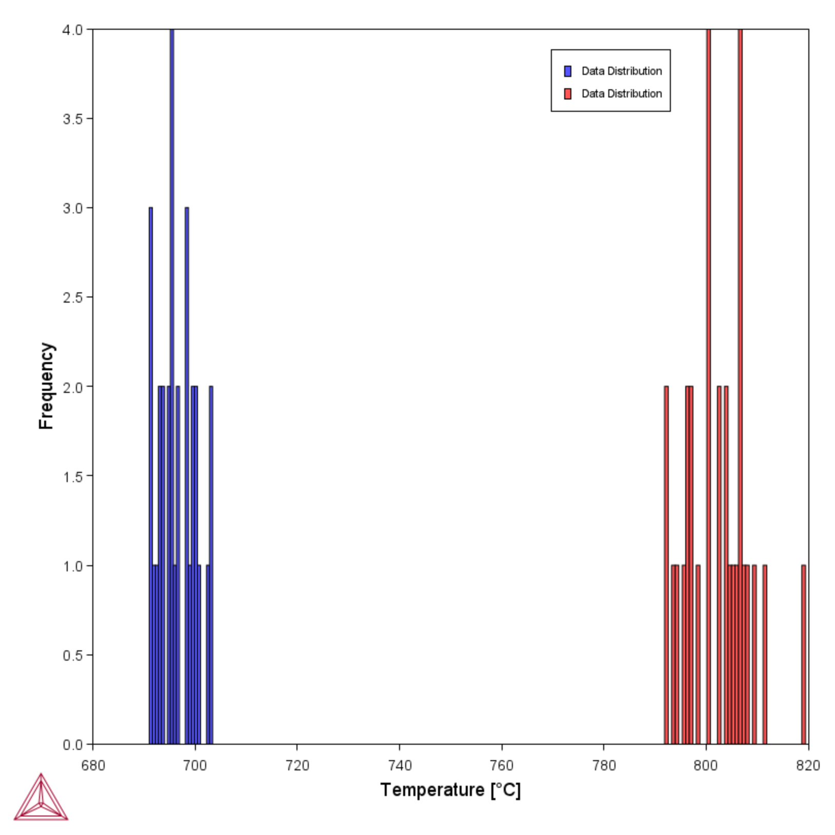
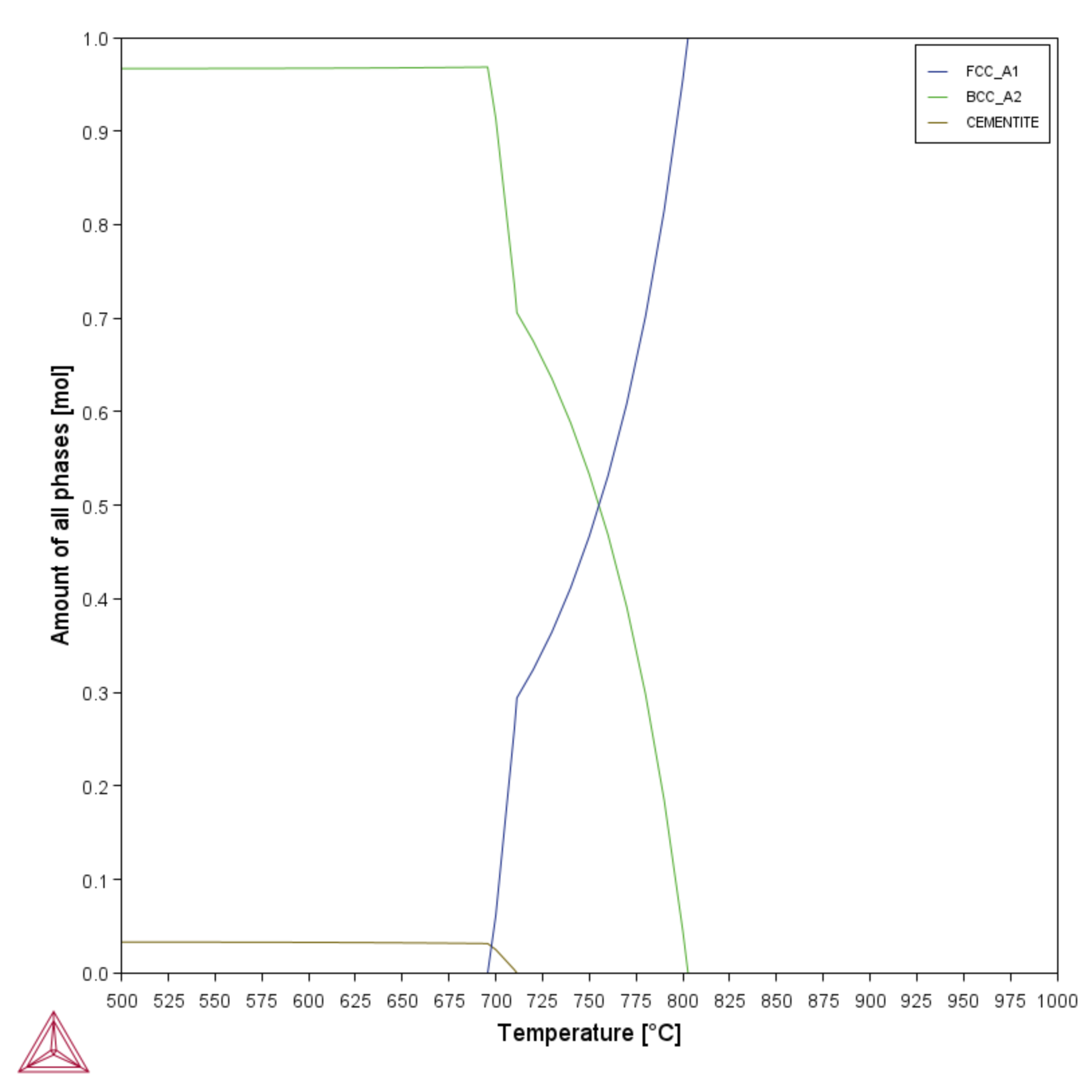
In the set up of the example, the Critical Transformation Temperatures model is used with a Property Model Calculator Uncertainty calculation to plot a histogram showing the distribution of A1- and A3-temperatures (Figure 1). As a comparison, an Equilibrium Calculator, One Axis calculation results in a property diagram showing the phase transitions for the nominal composition (Figure 2).
The phase transition temperatures are defined as:
- Liquidus: First austenite or ferrite transformation from the liquid
- Solidus: Liquid fully transformed to solid
- A0: Magnetic transition temperature (Curie temperature) of cementite. The cementite is paramagnetic above A0 and ferromagnetic below
- A1: Austenite (FCC_A1) transforms to ferrite (BCC_A2) + carbide (cementite or graphite or M23C6)
- A2: Magnetic transition temperature (Curie temperature) of ferrite (BCC_A2). Paramagnetic above A2 and ferromagnetic below
- A3: Austenite (FCC_A1) transforms to ferrite (BCC_A2)
Property Model Calculator and About the Critical Transformation Temperatures Property Model
- Folder: Property Models → Steel
- File name:
PM_Fe_04_Critical_Temperatures.tcu
The FEDEMO: Iron Demo Database is used and this example is available to all users. However, in general a license is required to run the Steel Models.
Visualizations
Many of our Graphical Mode examples have video tutorials, which you can access in a variety of ways. When in Thermo‑Calc, from the menu select Help → Video Tutorials, or from the main My Project window, click Video Tutorials. Alternately, you can go to the website or our YouTube channel.
Open the example project file to review the node setup on the Project window and the associated settings on the Configuration window for each node. For some types of projects, you can also adjust settings on the Plot Renderer Configuration window to preview results before performing the simulation. Click Perform Tree to generate plots and tables to see the results on the Visualizations window.

