D_04: Fe-C Moving Boundary - Austenite to Ferrite
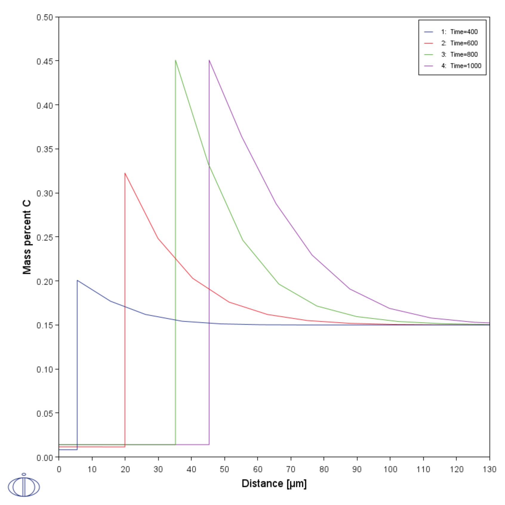
This example simulates the austenite to ferrite transformation in a Fe-0.01 mass% C steel during continuous cooling. The simulation starts at a temperature where only austenite is stable, ferrite nucleates and grows into the austenite during cooling in the two phase region. Plots of thermal and carbon composition profiles are generated.
- Folder: Diffusion Module - DICTRA
- File name:
D_04_Diffusion_Fe-C_Moving_Boundary_Austenite_to_Ferrite.tcu
Visualizations
Many of our Graphical Mode examples have video tutorials, which you can access in a variety of ways. When in Thermo‑Calc, from the menu select Help → Video Tutorials, or from the main My Project window, click Video Tutorials. Alternately, you can go to the website or our YouTube channel.
Open the example project file to review the node setup on the Project window and the associated settings on the Configuration window for each node. For some types of projects, you can also adjust settings on the Plot Renderer Configuration window to preview results before performing the simulation. Click Perform Tree to generate plots and tables to see the results on the Visualizations window.
There is a variety of information shown in the Visualizations window that can be viewed during configuration and after performing the calculation.
- Composition Profiles and Thermal Profile: When setting up a calculator on a Configuration window you can preview the profile and adjust settings as needed. When you click a calculator node in the Project window, the matching name of the node is on the tab(s) displayed in the Visualizations window.
- Plot or Table results: After completing the set up and performing the calculation, to view the matching name of the node on tab(s) in the Visualizations window, either click a Plot Renderer or Table Renderer node in the Project window or click the tabs individually in the Visualizations window.
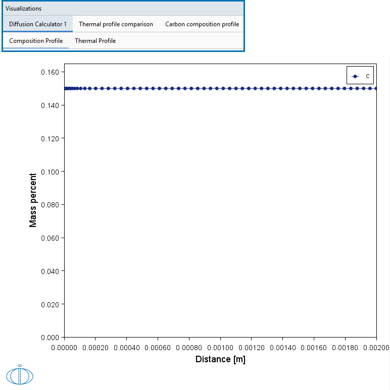
Figure 1: During set up of the calculation, preview the Composition Profile. Click the tab in the Visualizations window to switch between these previews and adjust settings on the Diffusion Calculator Configuration window.
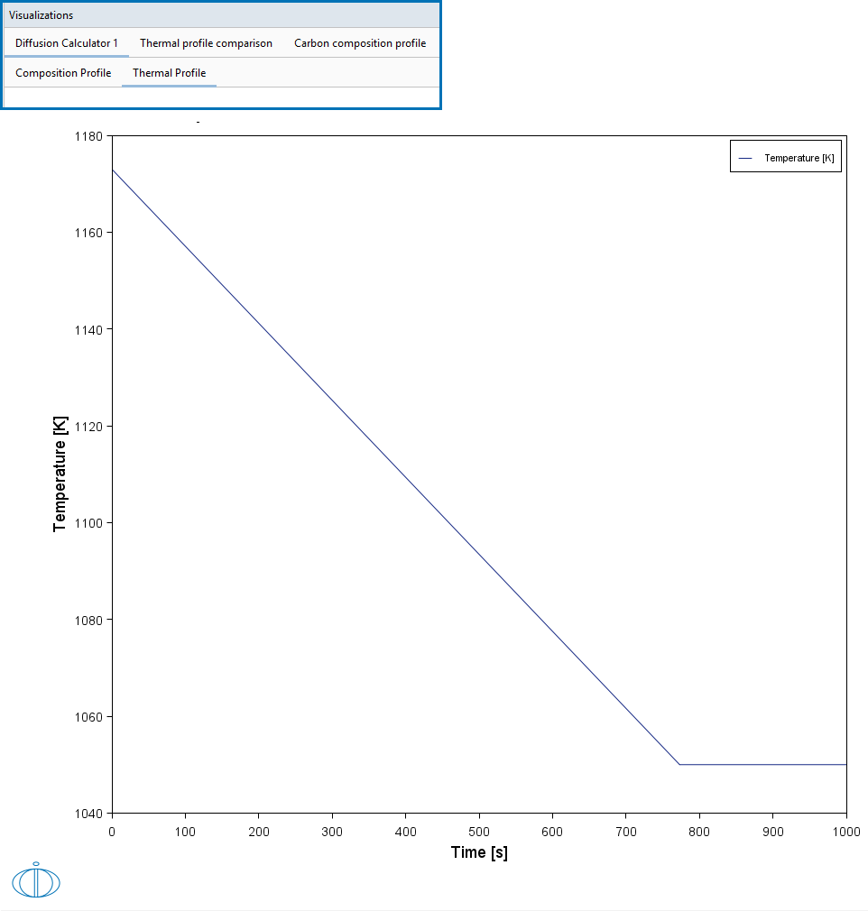
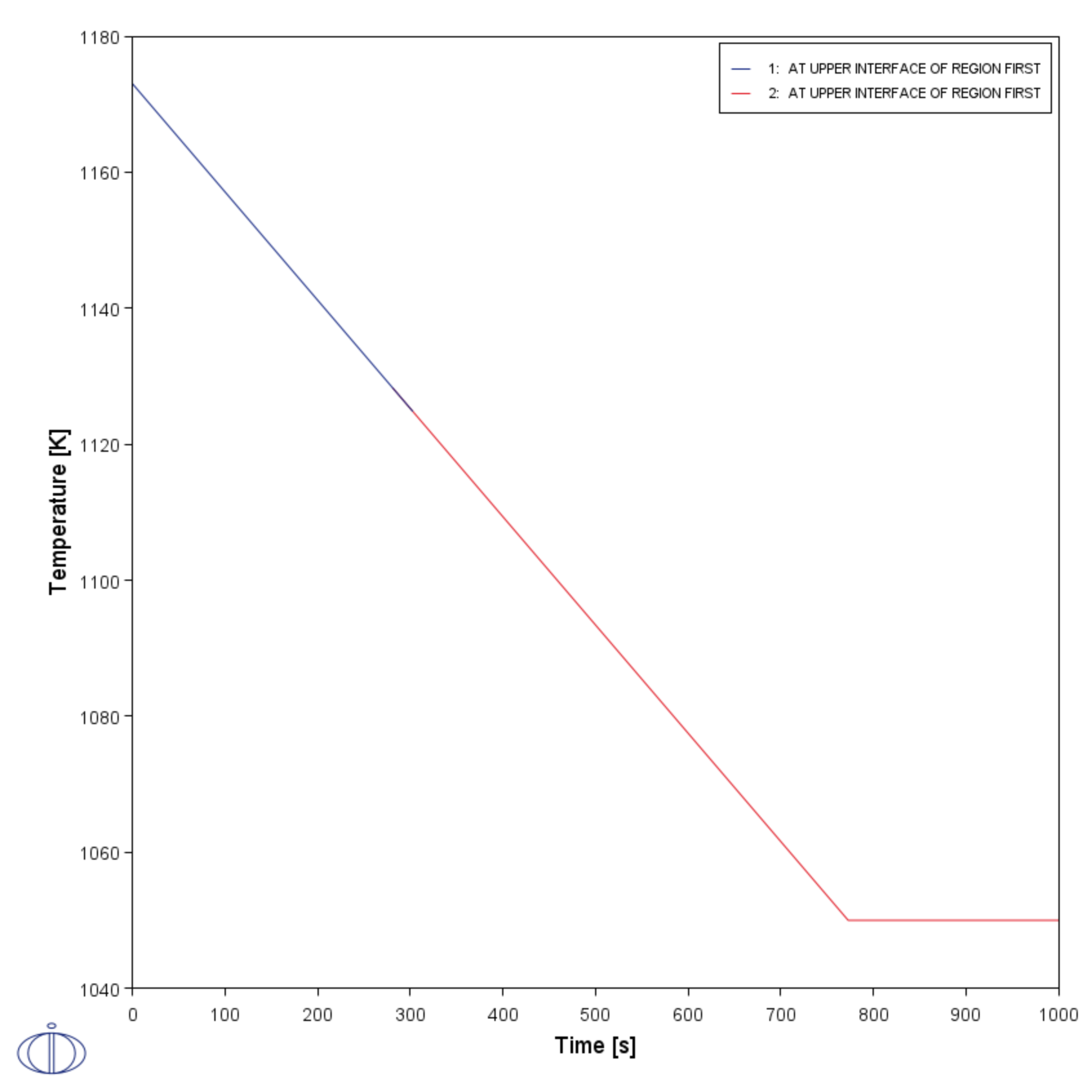
Figure 2: During set up of the calculation, preview the non-isothermal Thermal Profile. Click the tab in the Visualizations window to switch between these previews and adjust settings on the Diffusion Calculator Configuration window. Also see the plot result comparing the thermal profile for the two regions.
Figure 3: After performing the calculation, view the result on the Thermal profile tab. In this example, the Plot Renderer is renamed and this matches the tab name in the Visualizations window. Note that this Thermal Profile is slightly different than what you can preview during set up.


