D_09: Ni Post Weld Heat Treatment
In this example, a Ni-based alloy (Ni-Al-Co-Cr-Mo-Ti) post weld heat treatment analysis is completed. It shows how to import an initial composition profile from a file into the Diffusion Calculator. Then the calculation is run and plotted to show the composition of Al vs distance compared to experimental data from [2017She]. Such simulations can be used to design the heat treatment such that the desired homogenization of the weld is achieved. The initial composition profile needs to be determined by suitable experimental techniques, for example microprobe.
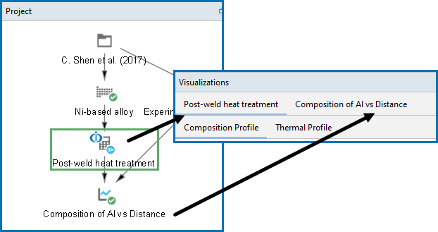
This example highlights the dual purpose of the Visualizations window where you can enter or import Composition profiles via the Diffusion Calculator Configuration window as well as being able to view and analyze results via the Plot Renderer after a calculation runs.
Visualizations
Many of our Graphical Mode examples have video tutorials, which you can access in a variety of ways. When in Thermo‑Calc, from the menu select Help → Video Tutorials, or from the main My Project window, click Video Tutorials. Alternately, you can go to the website or our YouTube channel.
Open the example project file to review the node setup on the Project window and the associated settings on the Configuration window for each node. For some types of projects, you can also adjust settings on the Plot Renderer Configuration window to preview results before performing the simulation. Click Perform Tree to generate plots and tables to see the results on the Visualizations window.
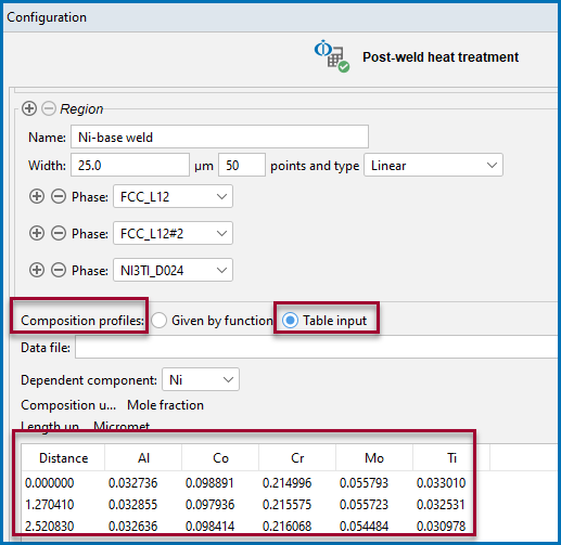
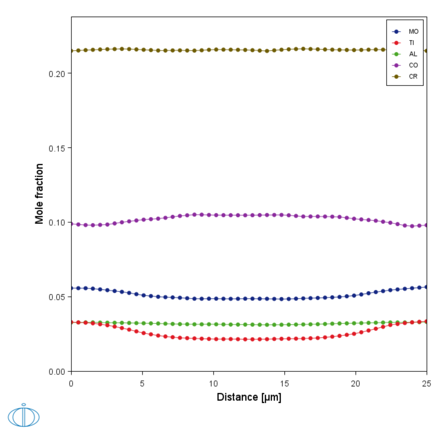
On the Diffusion Calculator, when defining its setup, the Composition profiles are imported using the Table input option. A prepared file, in this case a csv file, is set up with the correct data columns, which then are included on the Configuration window. After import the Composition Profiles are further able to be seen via the Visualizations window, at which point adjustments can be made as needed. In this isothermal example, you can also see that the constant temperature of the Thermal Profile is previewed.
Composition Profiles and Diffusion Calculator Thermal Profile for details about these settings and how to correctly set up files to import.
Figure 1: The Diffusion Calculator Configuration window showing the composition profile data, which is then compiled and displayed on the Visualizations window.
Figure 2: The Visualizations window displays details from both the Diffusion Calculator node (renamed to Post-weld heat treatment) via the Composition Profile and Thermal Profile tabs as well as the Plot Renderer node (renamed to Composition of Al vs Distance).
Figure 3: The Composition Profiles as shown in the Visualizations window after data is prepared and then imported into the Diffusion Calculator Configuration window.
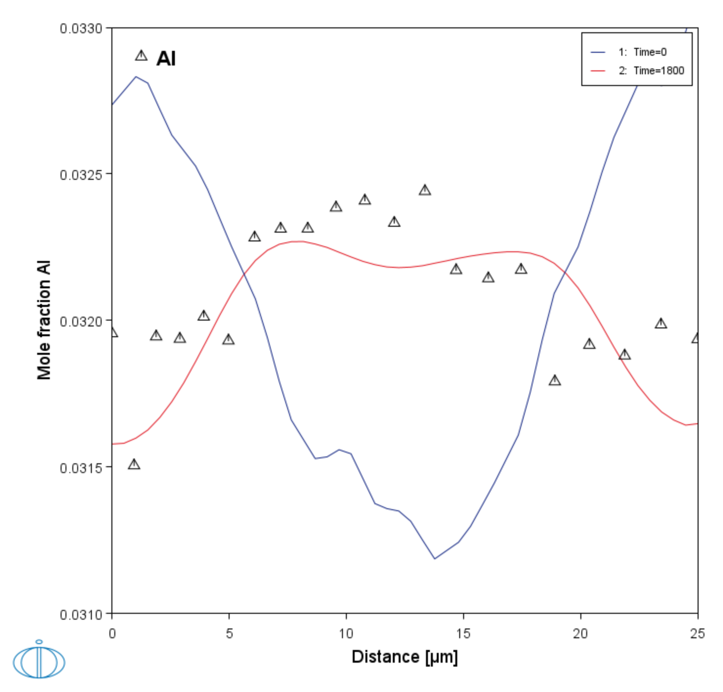
An Experimental File Reader node is used to supply experimental data from [2017She] to the Plot Renderer to validate the composition of, for example, Al vs distance on the Plot Renderer. The plot shows the content of Al along the cross-section of the weld, both before and after the post weld heat treatment. There is good agreement between the diffusion simulation and the data measured in the literature.
Figure 4: Plot results showing the mole fraction of Al before and after the heat treatment as a function of distance for a Ni-based alloy compared to experimental data [2017She].
Other plots can be added to investigate further details of the simulations, such as phase fractions or compositions.
Reference
[2017She] C. Shen, V. Gupta, S. Huang, M. Soare, P. Zhao, Y. Wang, “Modeling Long-term Creep Performance for Welded Nickel-base Superalloy Structures for Power Generation Systems” (Pittsburgh, PA, and Morgantown, WV (United States), 2017).


