AM Plot Type: 3D Plot
The 3D Plot is available with all simulation types (Steady-state, Transient, and Transient with heat source from Steady-state). It is also available with Steady-state calculation types Heat Source Calibration, Batch, and Grid.
The 3D Plot type has its own tab on both the Plot Renderer Configuration window and the Visualizations window. This plot type is further visualized using additional Display options.
Further, when connecting two AM Calculators to plot combinations of axis variables, separate tabs are added to the Visualizations window that have a suffix of the name of the AM Calculator added in brackets, e.g. 3D Plot (AM Calculator 1). It is recommended that the AM Calculator is renamed to help you identify which tab belongs to which calculation.
See Overlaying Plots in the AM Module for more details and AM Plot Type: Thermal Gradient vs. Solidification Rate for an example.
3D Plot Display Options
The Display options available are also based on the Axis variable selected. The Slice plot, which is a unique type of plot, is also available when either Surface colormap or Contour is selected.
Surface colormap, Contour, and Iso-surface are available when Temperature, Surface tension, Thermal conductivity, or Dynamic viscosity is selected as an Axis variable.
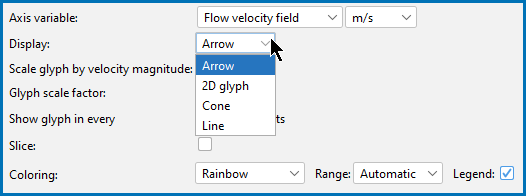
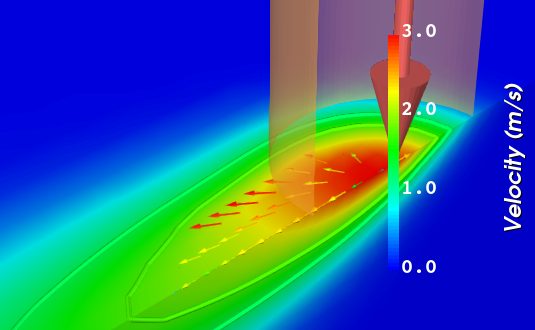
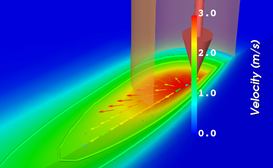
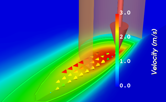
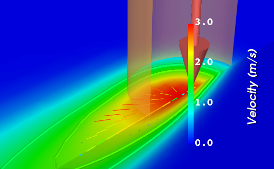
Arrow, 2D Glyph, Cone, or Line are available when Flow velocity field is selected as an Axis variable. It also requires that the Fluid flow including Marangoni effect checkbox is also selected on the AM Calculator.
Examples
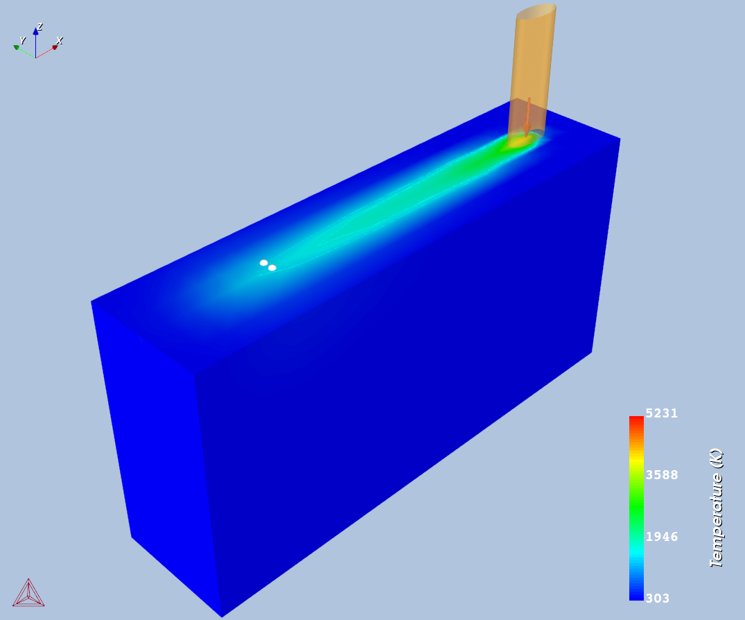
This is an example from AM_01: Transient Simulation of a Single Track.
This is an example from AM_01: Transient Simulation of a Single Track.
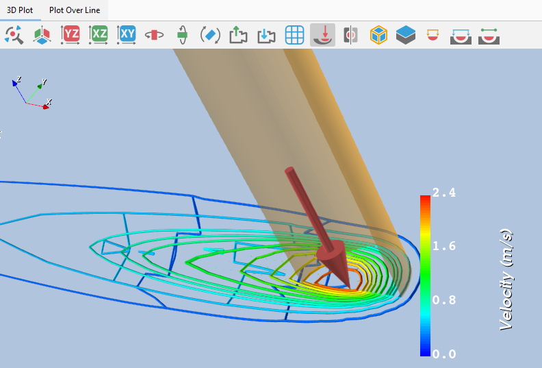
This is an example using AM_03: Steady-state Simulations to zoom into the AM Calculator, which in that example is renamed to Gaussian HS, with Fluid. On the Plot Renderer, the Display setting is changed from the default to Contour.
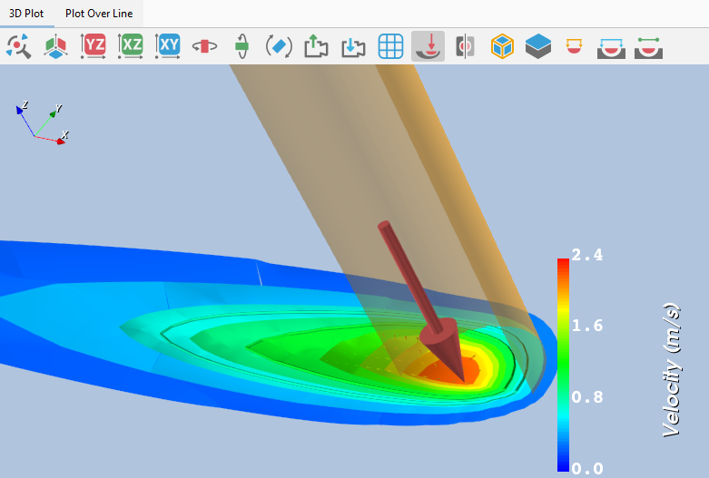
This is an example using AM_03: Steady-state Simulations to zoom into the AM Calculator, which in that example is renamed to Gaussian HS, with Fluid. On the Plot Renderer, the Display setting is changed from the default to Iso-surface.
This is an example using AM_04: Scheil Transient Steady-state to zoom into one of the AM Calculators, which in this case is renamed to Steady-state. On the Plot Renderer, and when the Axis variable is set to Flow velocity field, the Display default setting is Arrow.
This is an example using AM_04: Scheil Transient Steady-state to zoom into one of the AM Calculators, which in this case is renamed to Steady-state. On the Plot Renderer, and when the Axis variable is set to Flow velocity field, the Display setting is changed from the default to 2D Glyph.
This is an example using AM_04: Scheil Transient Steady-state to zoom into one of the AM Calculators, which in this case is renamed to Steady-state. On the Plot Renderer, and when the Axis variable is set to Flow velocity field, the Display setting is changed from the default to Cone.
This is an example using AM_04: Scheil Transient Steady-state to zoom into one of the AM Calculators, which in this case is renamed to Steady-state. On the Plot Renderer, and when the Axis variable is set to Flow velocity field, the Display setting is changed from the default to Line.

