AM Plot Type: Parity Plot
This topic describes the plot type Parity Plot which is available with Batch calculations for a Steady-state simulation. This plot type is only to select on the Plot Renderer when the simulation uses the Batch Calculation Type with an AM Calculator.
These examples highlight the use of this plot: AM_07: Batch Calculations for an IN718 Alloy, AM_08b: Batch Calculations for a Ti64 Alloy and AM_09b: Batch Calculations for an SS316L Alloy.
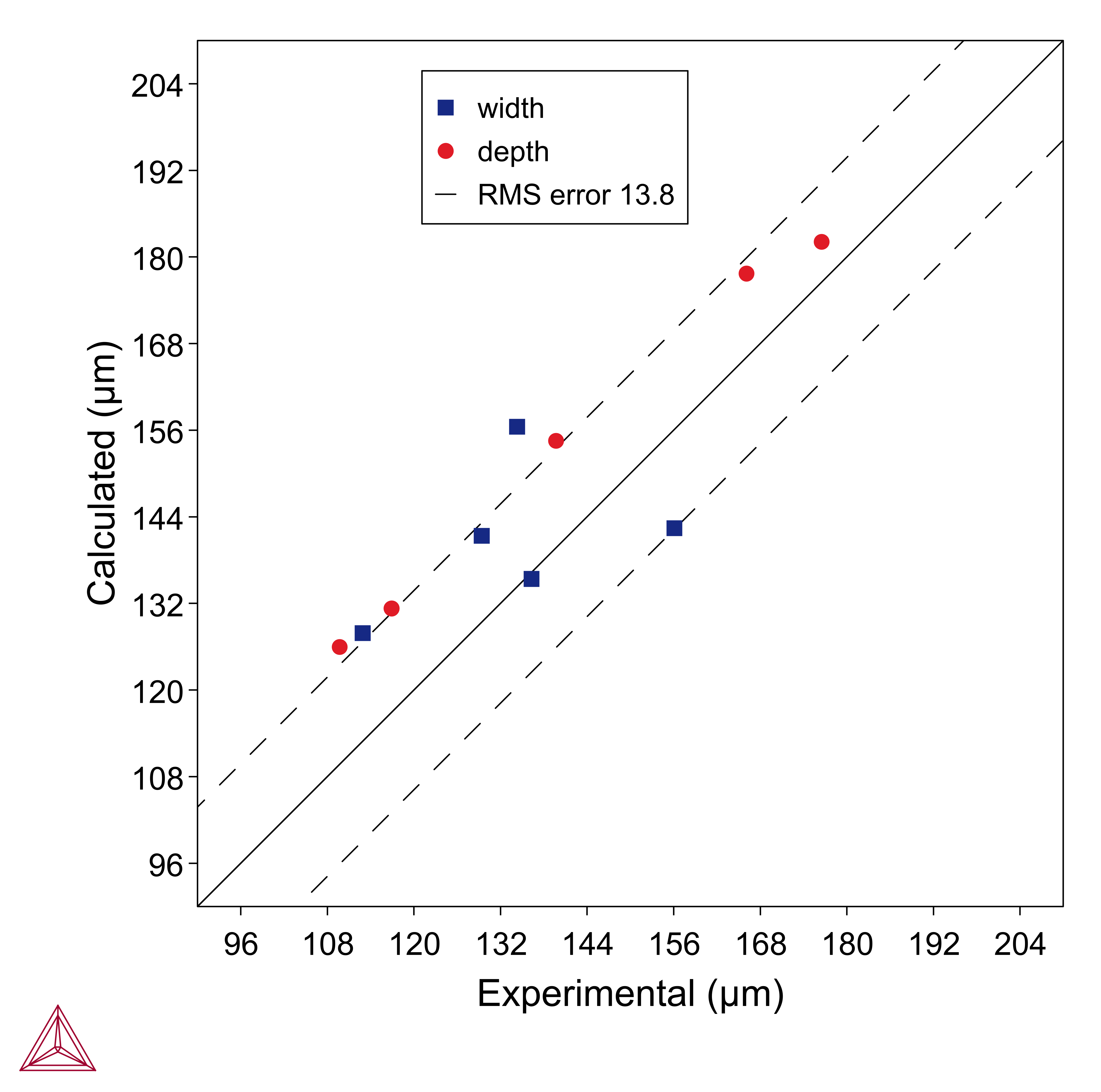
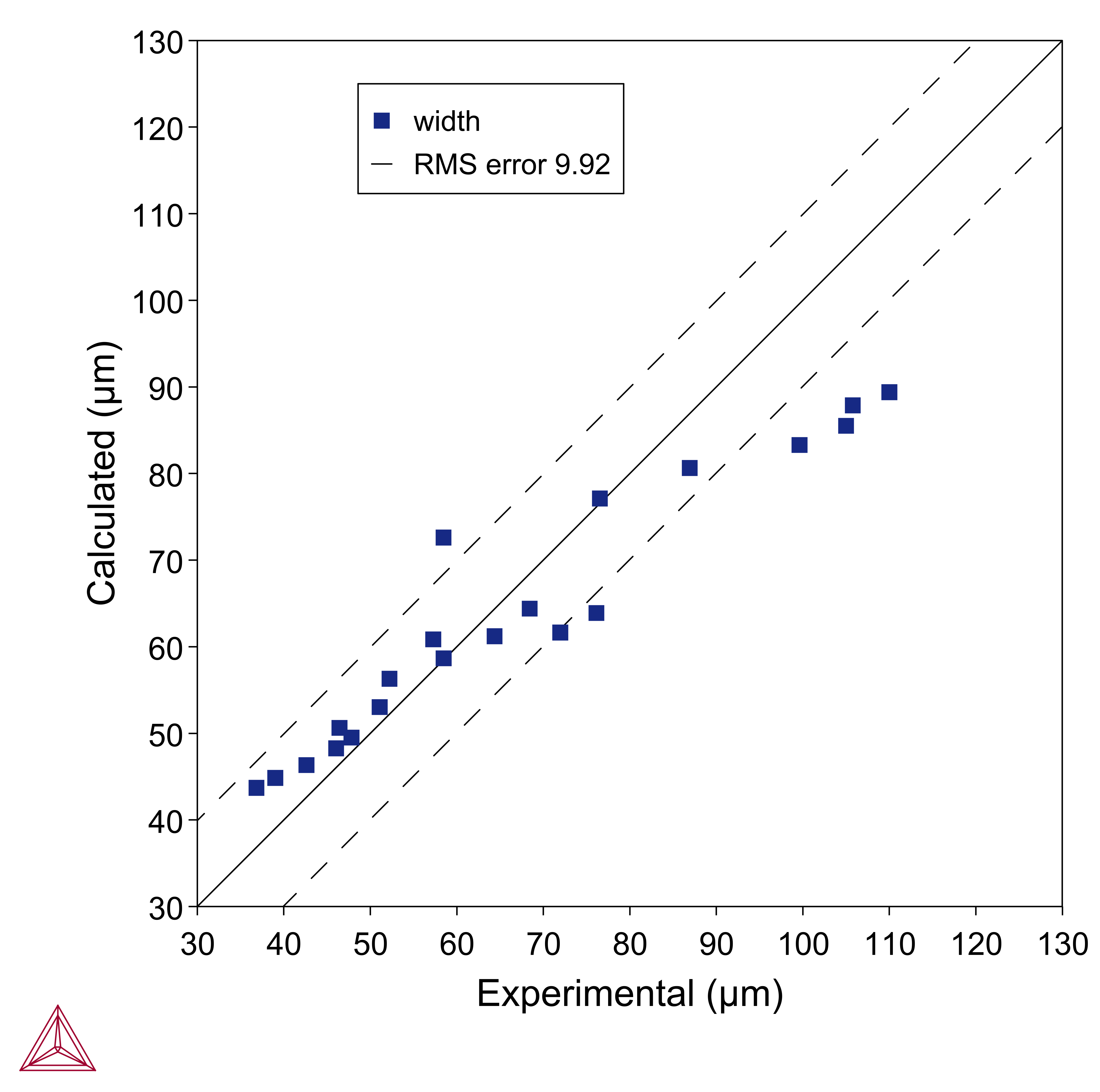
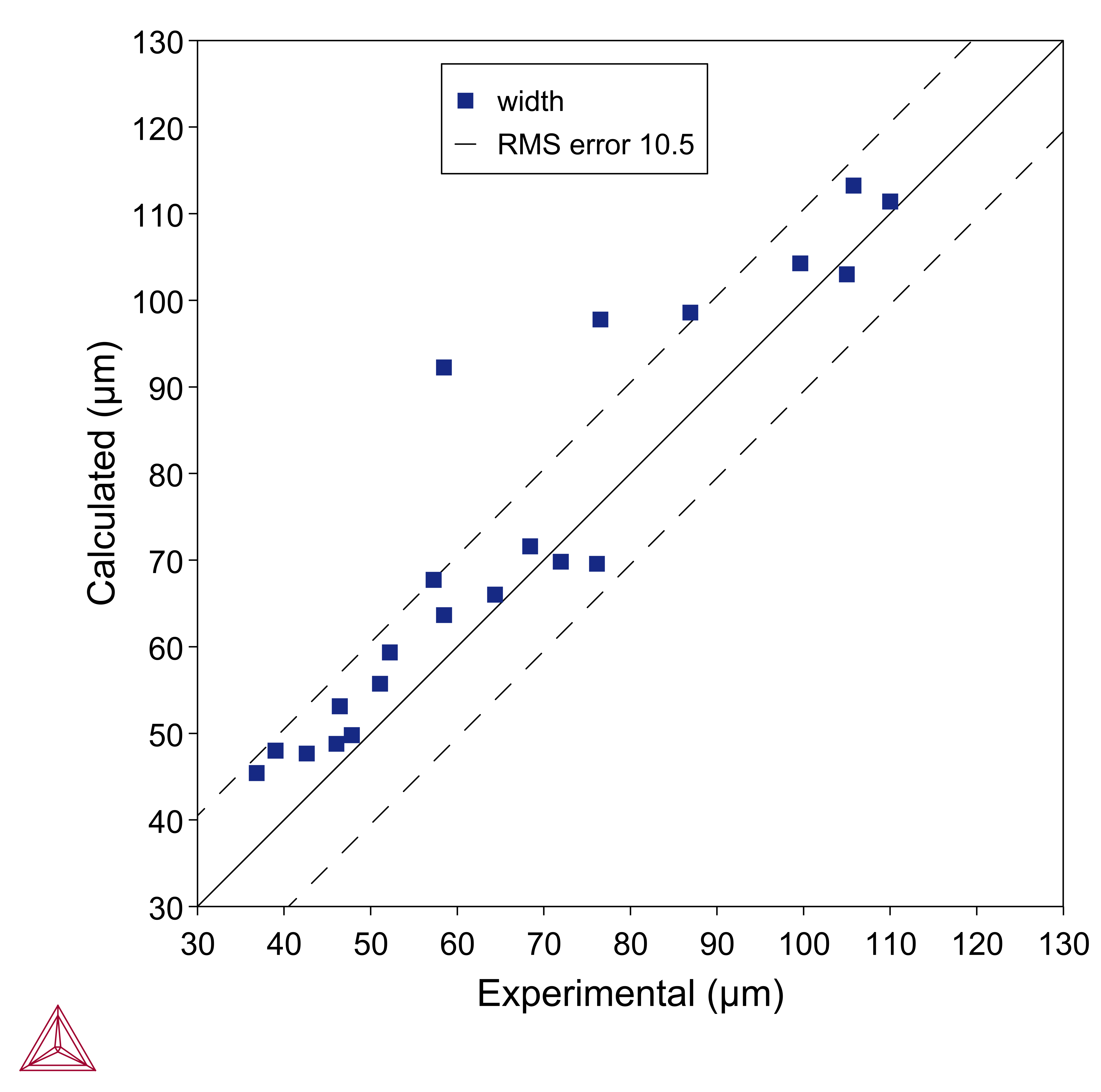
Parity plots are used when validating the Steady-state Batch calculation against experimentally measured melt pool width and depth. The plot shows the experimental width/depth on the X-axis and the calculated width/depth on the Y-axis. The data should follow the diagonal line for a perfect match between the calculated and experimental values.
The following are from example AM_07.
Figure 1: Parity plot comparing experimental versus calculated melt pool width and depth for all the experiments. The experiments are single tracks on bare plate IN718 with varied power and scan speed. The Root Mean Square (RMS) error can also be shown as a dashed line.
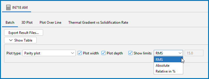
Figure 2: Alternatively, lines for user-defined Absolute or Relative in % error can be shown instead by selecting these options on the Configuration window.
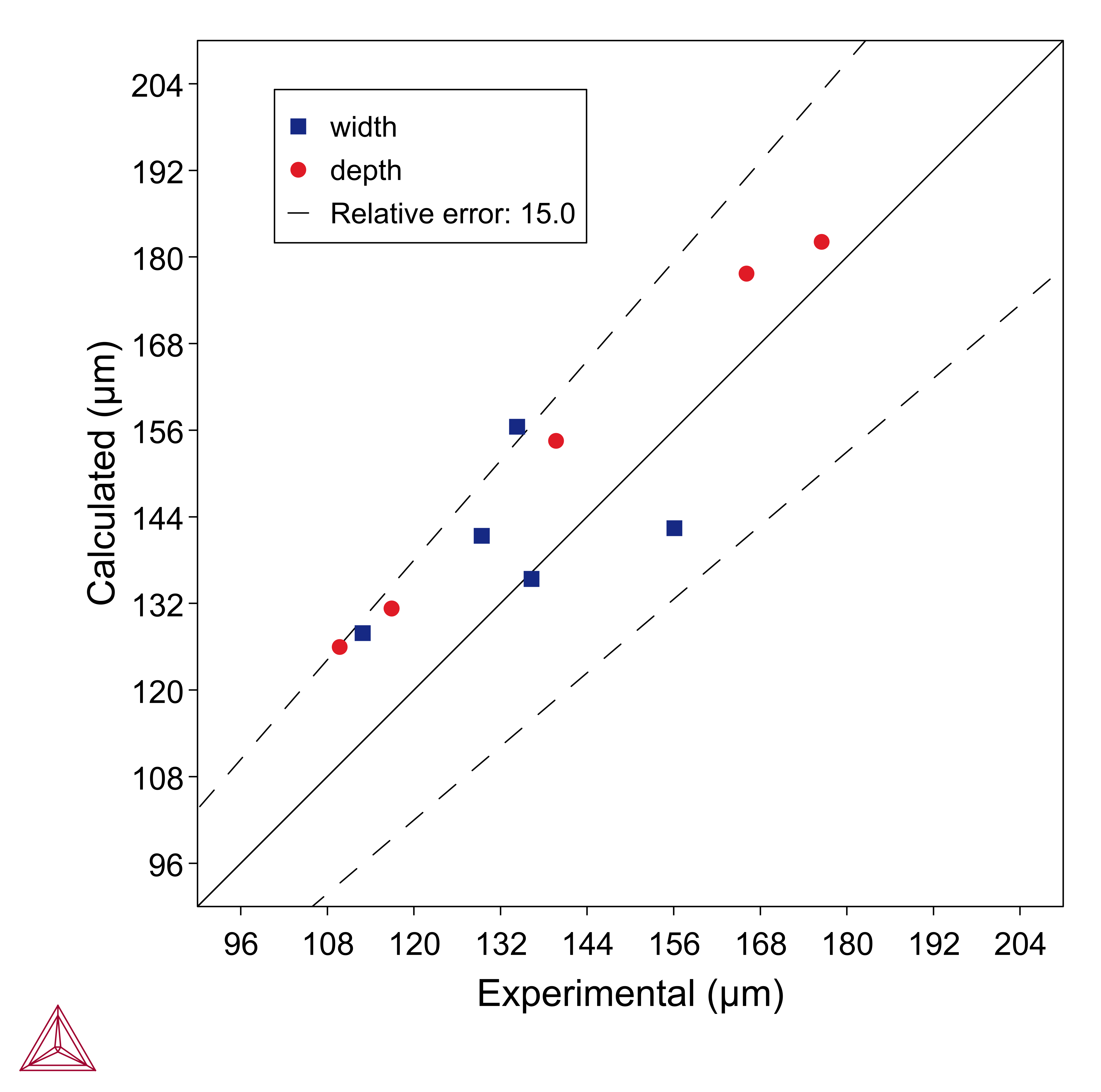
Figure 3: Parity plot comparing experimental versus calculated melt pool width and depth for all the experiments. The experiments are single tracks on bare plate IN718 with varied power and scan speed. In this plot, it is configured to show a Relative in % error of 5 instead of the RMS error.
Keyhole Model with Fluid Flow
This is an example application of using the parity plot when the keyhole model includes fluid flow, which can provide a better prediction of the melt pool size.
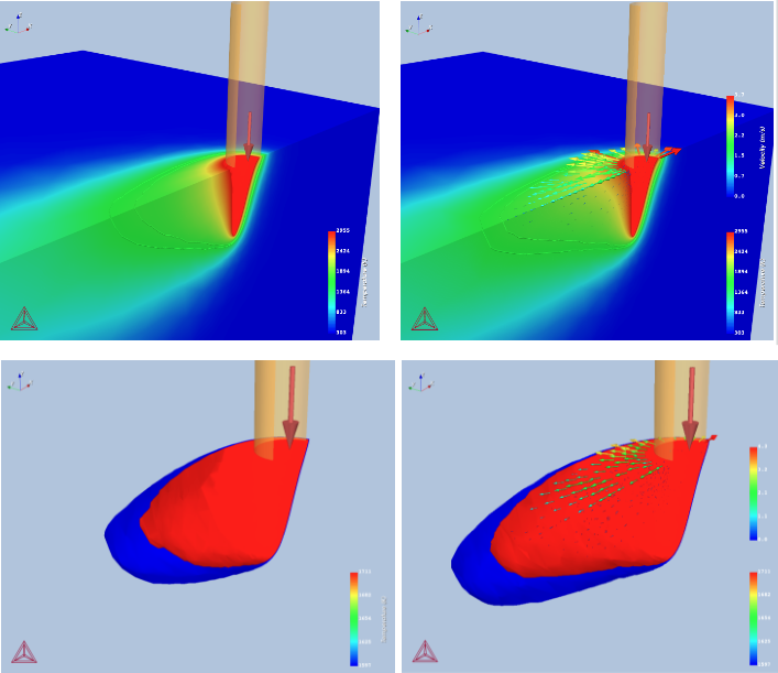
Keyholing can occur with low scanning speed and high power. Including fluid flow in the simulation makes the predictions of the entire melt pool size more accurate, which is especially important at higher energy densities when Marangoni forces are strong.
Figure 4: Fluid flow can make the melt pool wider and longer. This example shows the effect when enabling fluid flow for 316L for power 50 W and scan speed 400 mm/s. Left images show without fluid flow and right images with fluid flow enabled. Top row shows the temperature color map. Bottom row shows the isosurfaces for liquidus and solidus, i.e. the size of the melt pool and mushy zone.
|
|
Figure 5: Parity plot for 316L showing how the RMS is reduced for the melt pool width when excluding fluid flow (left) compared to when it is included (right). Experiments from Hu et. al [2019Hu].
Reference
[2019Hu] Z. Hu, B. Nagarajan, X. Song, R. Huang, W. Zhai, J. Wei, Formation of SS316L Single Tracks in Micro Selective Laser Melting: Surface, Geometry, and Defects. Adv. Mater. Sci. Eng. 2019, 1–9 (2019).
