AM_04: Scheil Transient Steady-state
In this example, three different simulations are performed: Steady-state, Transient Single track, and Transient Multilayer. Both Transient Single track and Transient Multilayer use Transient with heat source from Steady-state model to compute time-dependent temperature distribution in the given geometry. The primary difference between this example and the previous examples (AM_01 to AM_03) is that, in this case, the material properties data is retrieved from the Scheil Calculator whereas in the previous examples the material properties are taken from the preinstalled material library. Furthermore, this example simulates scanning of two layers of powder where the second layer is spread on the top of the first layer when scanning of the first layer is completed.
- Folder: Additive Manufacturing
- File name:
AM_04_Scheil_TransientSS.tcu
Material chosen for this example is Ti-6Al-4V. To run this example requires both version TCTI5.0 and newer of the TCS Ti/TiAl-based Alloys Database (TCTI) in addition to a license for the Additive Manufacturing (AM) Module. Some portions of this example are also covered in the Getting Started Guide on our website.
Visualizations
Open the example project file to review the node setup on the Project window and the associated settings on the Configuration window for each node. For some types of projects, you can also adjust settings on the Plot Renderer Configuration window to preview results before performing the simulation. Click Perform Tree to generate plots and tables to see the results on the Visualizations window.
When you run (Perform) this example, it takes at least 30 minutes for the calculations to complete.
There is a variety of information shown in the Visualizations window that can be viewed during configuration and after performing the calculation(s).
- Geometry: View the geometry and adjust parameters visually by changing inputs on the Configuration window.
- Melt pool and other dynamically changing features can also be visualized and changed.
- Plot results: After completing the set up and performing the calculation, to view the matching name of the node on tab(s) in the Visualizations window, click a Plot Renderer node in the Project window or click the tabs individually in the Visualizations window.
Steady-state
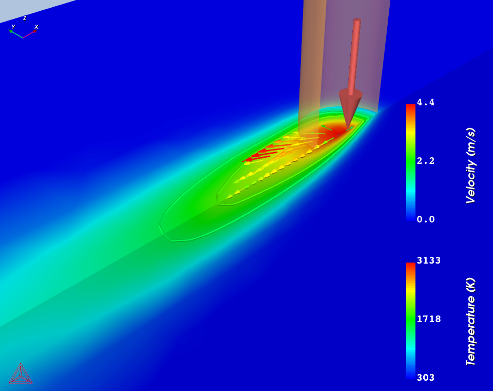
The Steady-state calculator of this example computes temperature distribution in a steady state for the power of 100 W and scanning speed of 600 mm/s. The beam radius in this example is taken as 100 μm. For the geometry, the steady-state model only needs the height of the solid substrate as the input, which is taken as 2.0 mm. The solid substrate is covered with a powder layer of thickness 55 μm. This example also takes into account the effect of fluid flow due to Marangoni forces inside the melt pool.
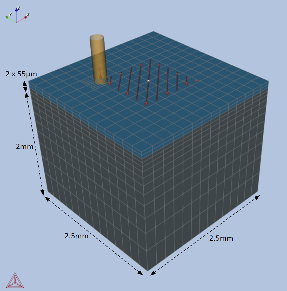
Figure 1: Geometry definition for Transient Multilayer. The scanning strategy shows the scanning pattern on the top most layer.
Figure 2: Temperature distribution around the melt pool and mushy zone for the Steady-state case. Velocity vectors representing the fluid flow inside the melt pool can also be seen.
Transient Single Track
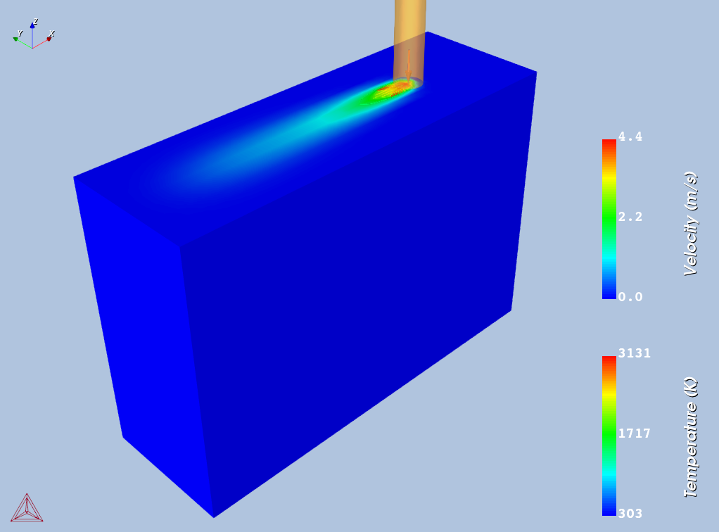
Figure 3: 3D Surface colormap showing temperature distribution at the end of single track transient simulation. The velocity vectors around the heat source show the direction of fluid flow in the melt pool.
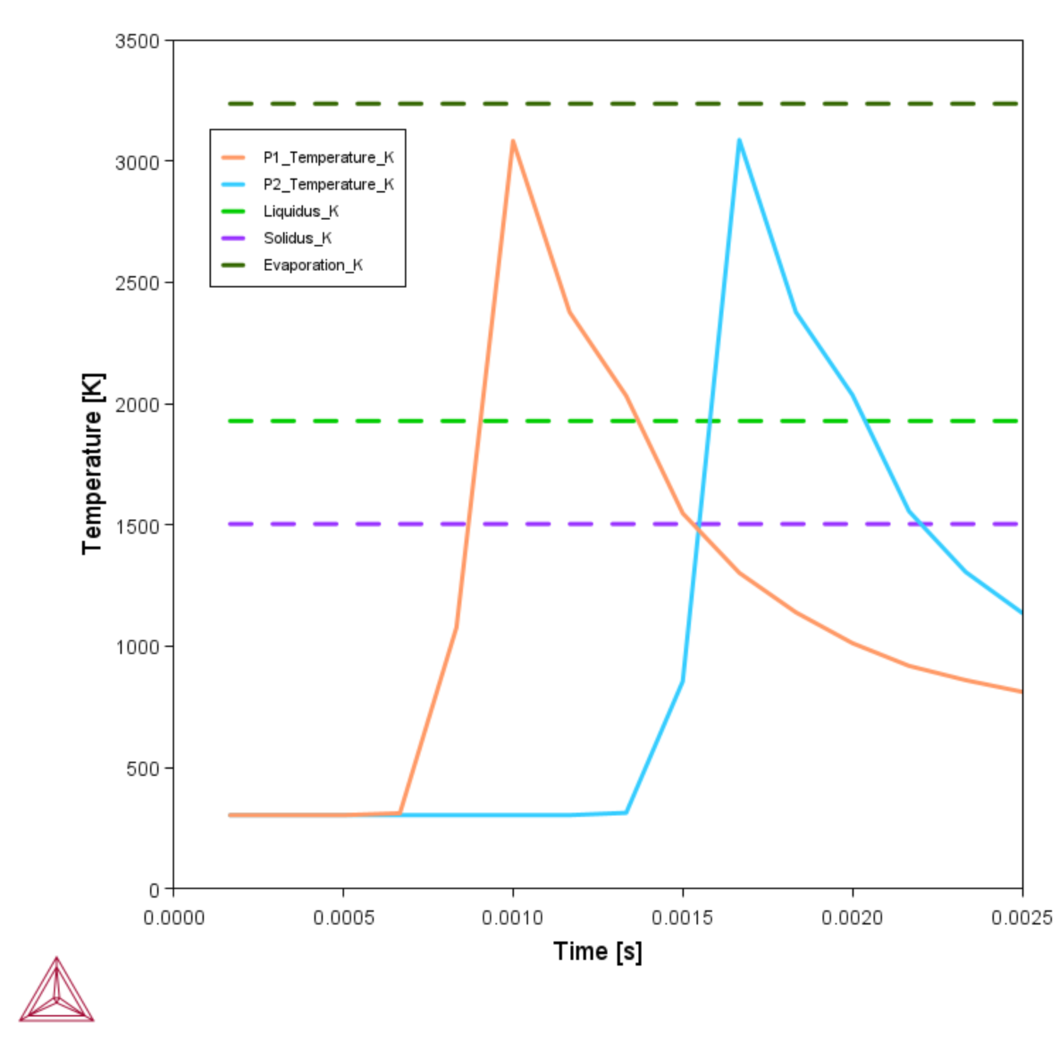
Figure 4: 2D Plot showing temperature as a function of time from Probe 1 (orange) and Probe 2 (blue) after the single track scan is completed.
Transient Multilayer
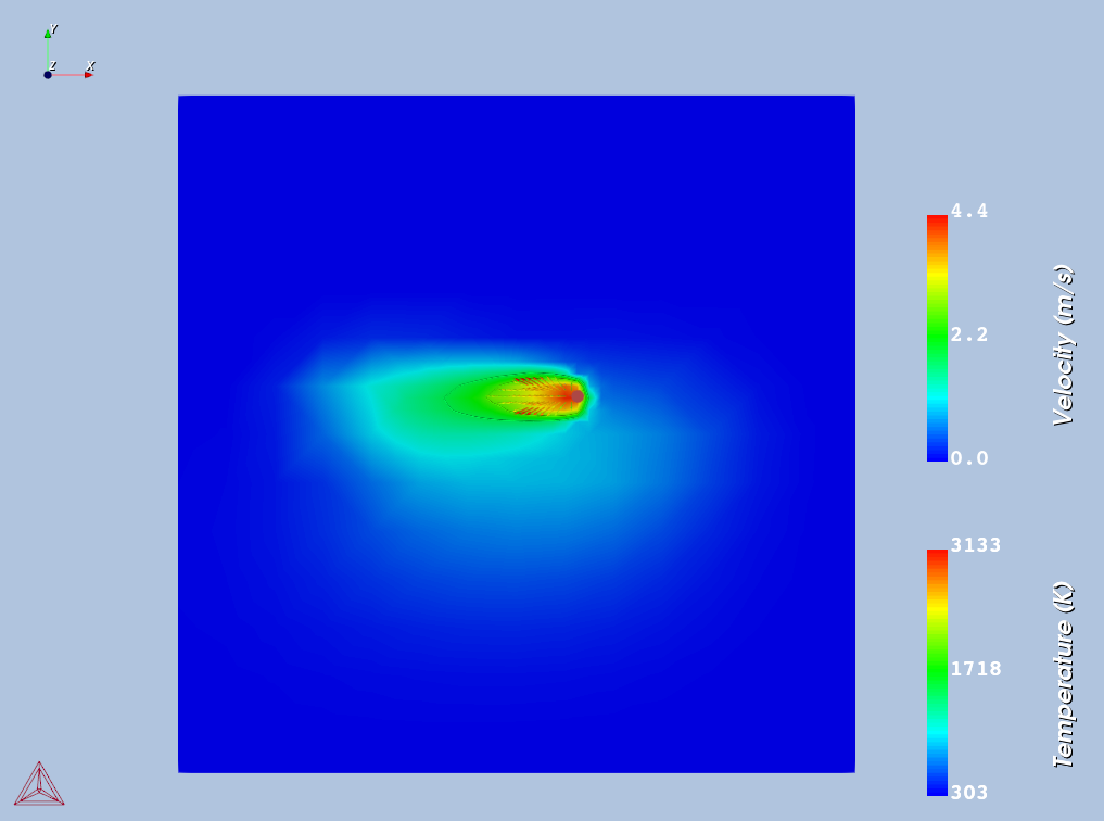
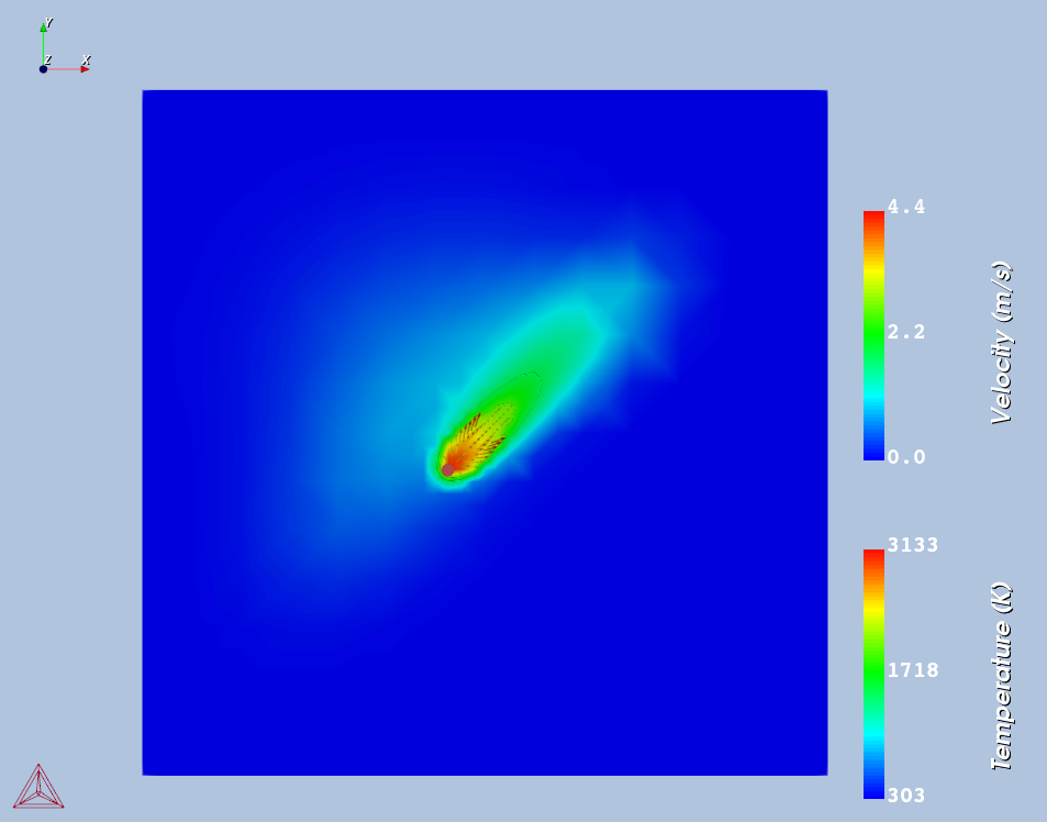
Figure 5: Temperature distribution on the top surface of the workpiece during scanning of the first layer.
Figure 6: Temperature distribution on the top surface of the workpiece during scanning of the second layer.
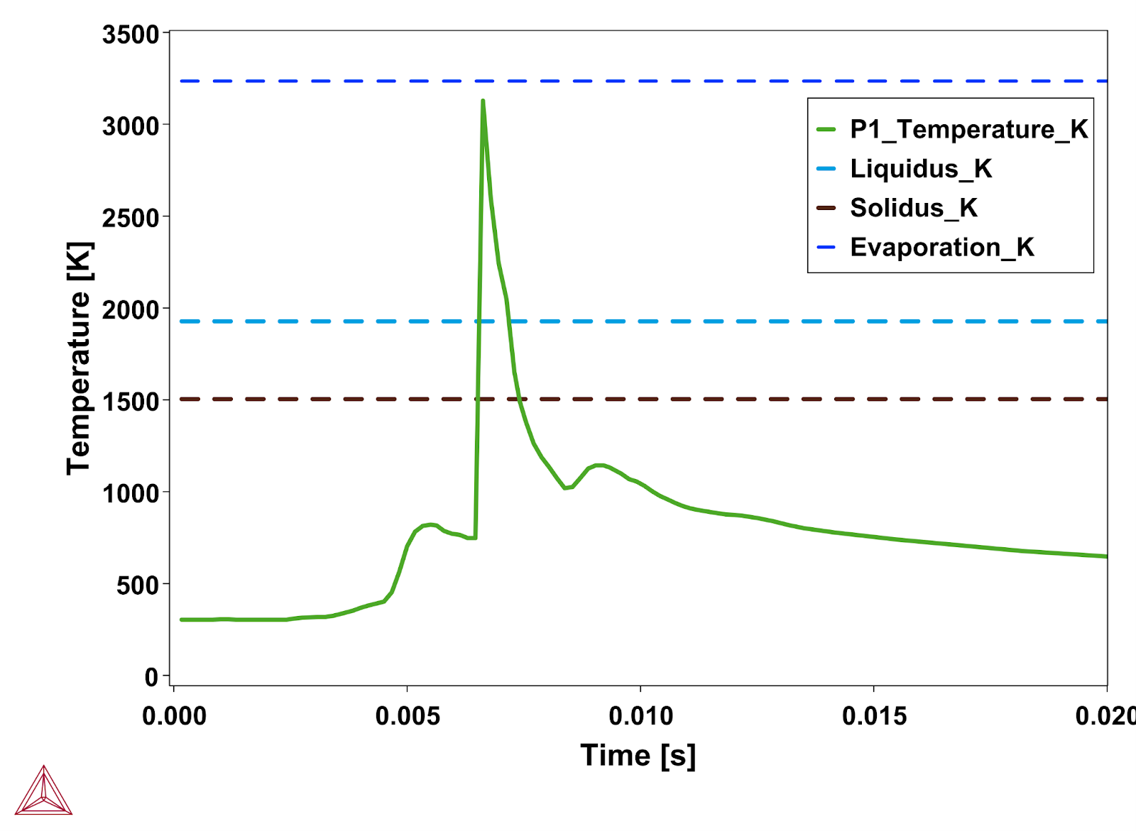
Figure 7: 2D Plot showing temperature as a function of time from Probe 1 after scanning the first layer.
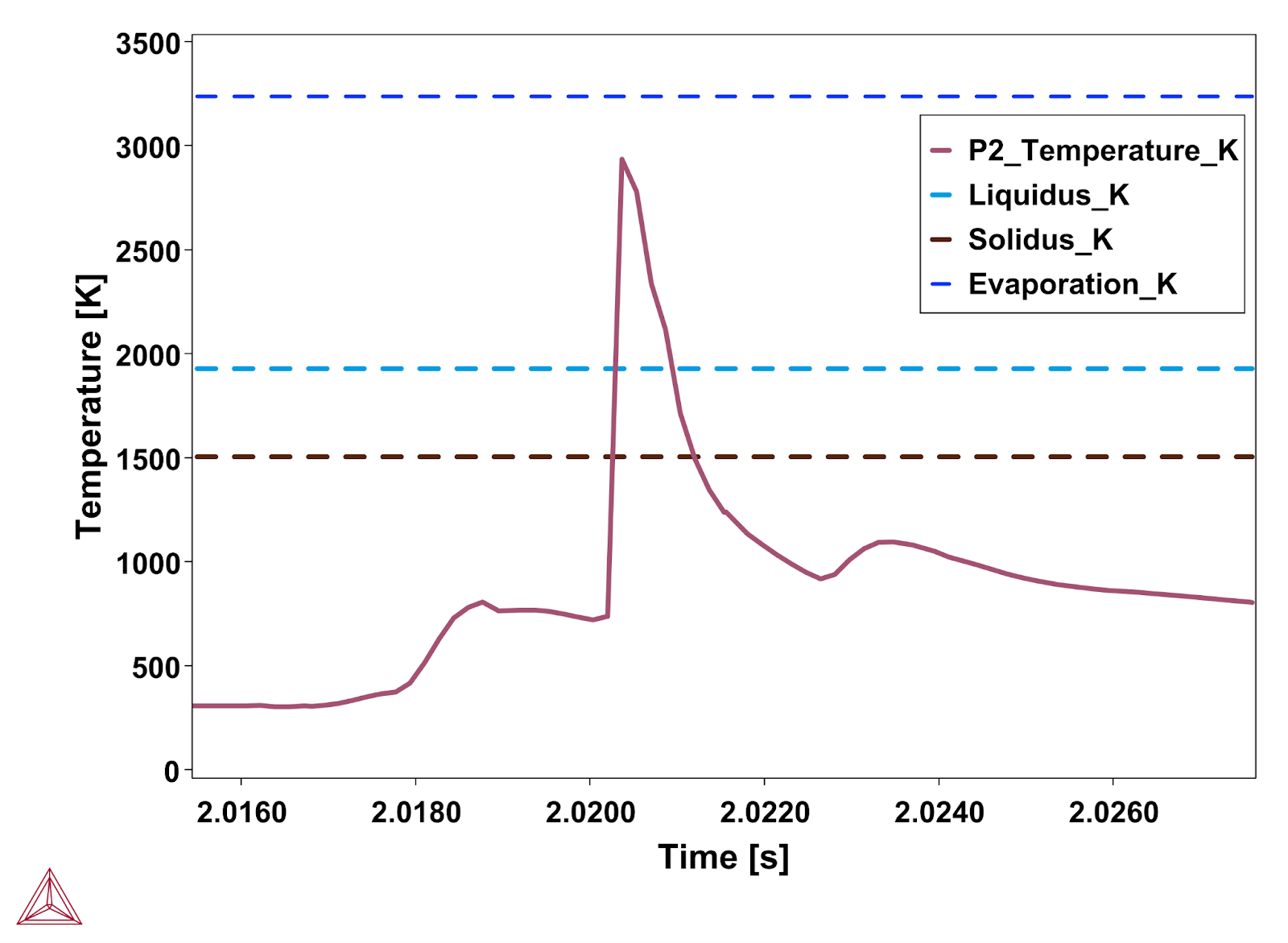
Figure 8: 2D Plot showing temperature as a function of time from Probe 2 after scanning the second layer.
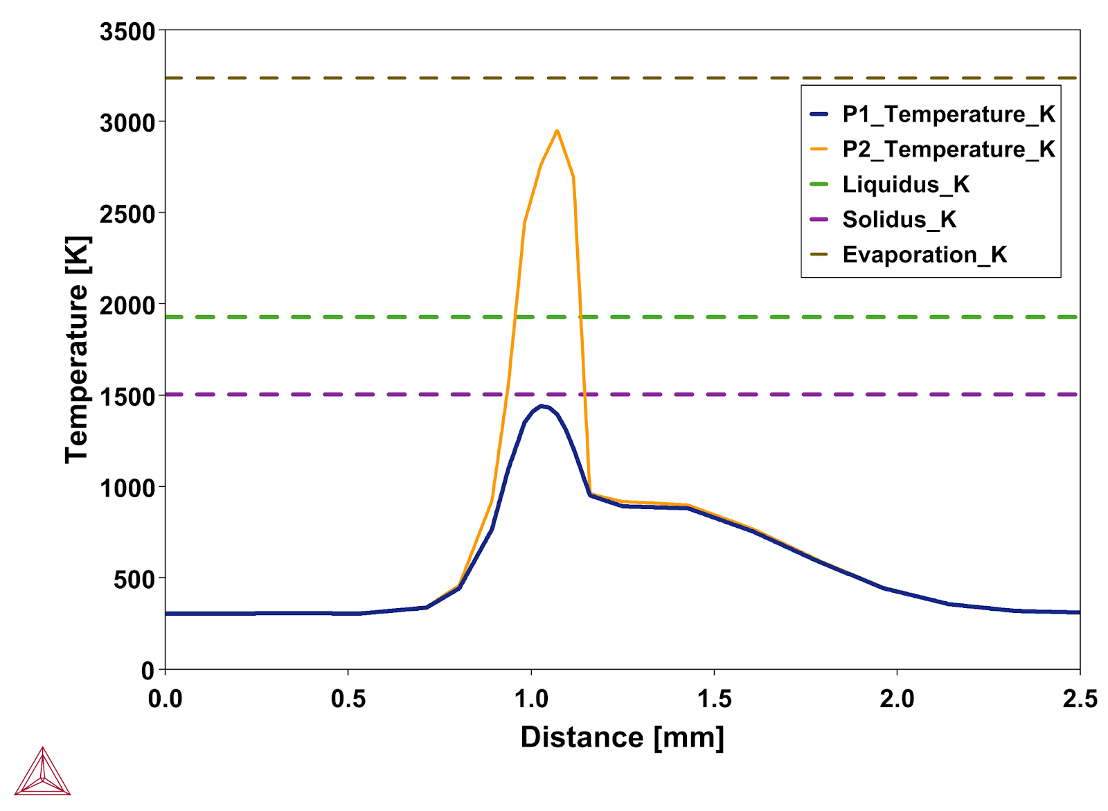
Figure 9: 2D Plot Over Line showing temperature profiles plotted along the lines, parallel to the width of the geometry placed on the top of the first layer (P1) and the second layer (P2).
Other Resources
Read more about the Additive Manufacturing (AM) Module on our website including the details about database compatibility or to watch an introductory webinar. You can also use the Getting Started Guide to learn about the key features available.
Many of our Graphical Mode examples have video tutorials, which you can access in a variety of ways. When in Thermo‑Calc, from the menu select Help → Video Tutorials, or from the main My Project window, click Video Tutorials. Alternately, you can go to the website or our YouTube channel.
