AM_07: Batch Calculations for an IN718 Alloy
This example shows the use of the AM Calculator with a Steady-state mode and Batch Calculation Type where it compares calculated and measured melt pool dimensions. The experimental data are from the 2022 NIST AM‑Bench Test Series [2022NIST] where single track experiments were performed on a IN718 bare plate at different power and scan speeds.
The use of different Plot types in this example include a Parity plot, 3D plot showing the keyhole, and Printability map.
This example is part of a set using a Steady-state simulation with a Gaussian heat source, plus the Keyhole model including Fluid flow. These examples collectively show the use of Batch and Grid calculation types plus various plot types such as Printability maps, Parity plots, and Melt pool vs energy density. The examples are numbered AM_07 to AM_09b.
- Folder: Additive Manufacturing
- File name:
AM_07_Batch_IN718.tcu
This example requires an Additive Manufacturing (AM) Module license.
Some examples (AM_01, AM_02, AM_03, and AM_06b) are available to all users. These examples can be run without an additional Additive Manufacturing license when you are in DEMO (demonstration) mode. However, the AM Module is not available with the Educational version of Thermo-Calc.
Configuration and Calculation Set Up
Below highlights the main settings for this example.
The Steady-state simulation is selected and the Fluid flow including Marangoni effect checkbox is selected.

The Heat Source is set to Gaussian and uses the Keyhole model. The printers in the experiments had a beam diameter of 67 μm so the Gaussian Beam radius is set to 33.5 μm. The Absorptivity is set to 30.0 %.

The IN718 material is selected from the Material Properties library. The material properties are precalculated and stored as a built-in material Library.

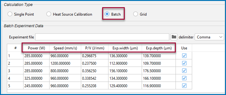
The Batch Calculation Type is used to set up all the conditions from the multiple experiments in a single calculation. The experimental Power and scan Speed as well as the measured melt pool Width and Depth were collected in a CSV file and read into the software. This data is then saved in the project file.
In the Batch Experiment Data table you can see that the power ranges between 245 W to 285 W and the scan speed ranges between 800 mm/s to 1200 mm/s.
Visualizations
Open the example project file to review the node setup on the Project window and the associated settings on the Configuration window for each node. For some types of projects, you can also adjust settings on the Plot Renderer Configuration window to preview results before performing the simulation. Click Perform Tree to generate plots and tables to see the results on the Visualizations window.
When you run (Perform) this example, it takes at least 30 minutes for the calculations to complete.
There is a wide variety of information shown both in the Visualizations and Plot Renderer Configuration windows that can be viewed during configuration and after performing the calculation(s). Not all views, such as the Geometry or previews, nor all additional output (i.e. plots) are shown in this section and it is recommended that you open and run the example to review all available options and results.
Parity Plot

Figure 1: Parity plot comparing experimental versus calculated melt pool width and depth for all the experiments. The experiments are single tracks on bare plate IN718 with varied power and scan speed. The Root Mean Square (RMS) error can also be shown as a dashed line.

Figure 2: Alternatively, lines for user-defined Absolute or Relative in % error can be shown instead by selecting these options on the Configuration window.
3D Plot with Surface Colormap

Figure 3: 3D plot showing a keyhole for the second simulation that uses power 285 W and scan speed 1200 mm/s.

Figure 4: Selecting the Batch experiment number to display in the Visualizations window for the 3D plot shown in Figure 3.
Visualizing Batch Calculations in the AM Module
Reference
[2022NIST] National Institute of Standards and Technology (NIST), Additive Manufacturing Benchmark Test Series (AM-Bench) (2022), (available at https://www.nist.gov/ambench).
Other Resources
Read more about the Additive Manufacturing (AM) Module on our website including the details about database compatibility or to watch an introductory webinar. You can also use the Getting Started Guide to learn about the key features available.
Many of our Graphical Mode examples have video tutorials, which you can access in a variety of ways. When in Thermo‑Calc, from the menu select Help → Video Tutorials, or from the main My Project window, click Video Tutorials. Alternately, you can go to the website or our YouTube channel.