Visualizing Heat Source Calibrations
This topic describes both the AM Calculator and the Plot Renderer visualization outcomes related to the heat source calibration calculations for a Steady-state simulation.
To import data for use in batch calculations, it is recommended you review AM Calculator Experiment File Requirements. Also review Working with AM Visualizations, which provides an overview of how most of the windows are connected.
It is recommended to open and run one of the examples to best understand the wide variety of visualization outcomes.
AM_06a: Calibrating a Heat Source for a 316L Steel and AM_06b: Using the Calibrated Heat Source for a 316L Steel
Working with AM Calculator Heat Source Calibration Experiment Data
During the set up of the Heat Source Calibration, experiment data is either entered or imported to the AM Calculator table where it is visible on its associated Configuration window.
Click the relevant AM Calculator node in the Project window to preview the table data via a Heat Source Calibration tab on the Visualizations window.
Use the table's Use column on the AM Calculator Configuration window to select the relevant checkboxes for which Width and Depth points to include (i.e. use) or exclude (i.e. not use).
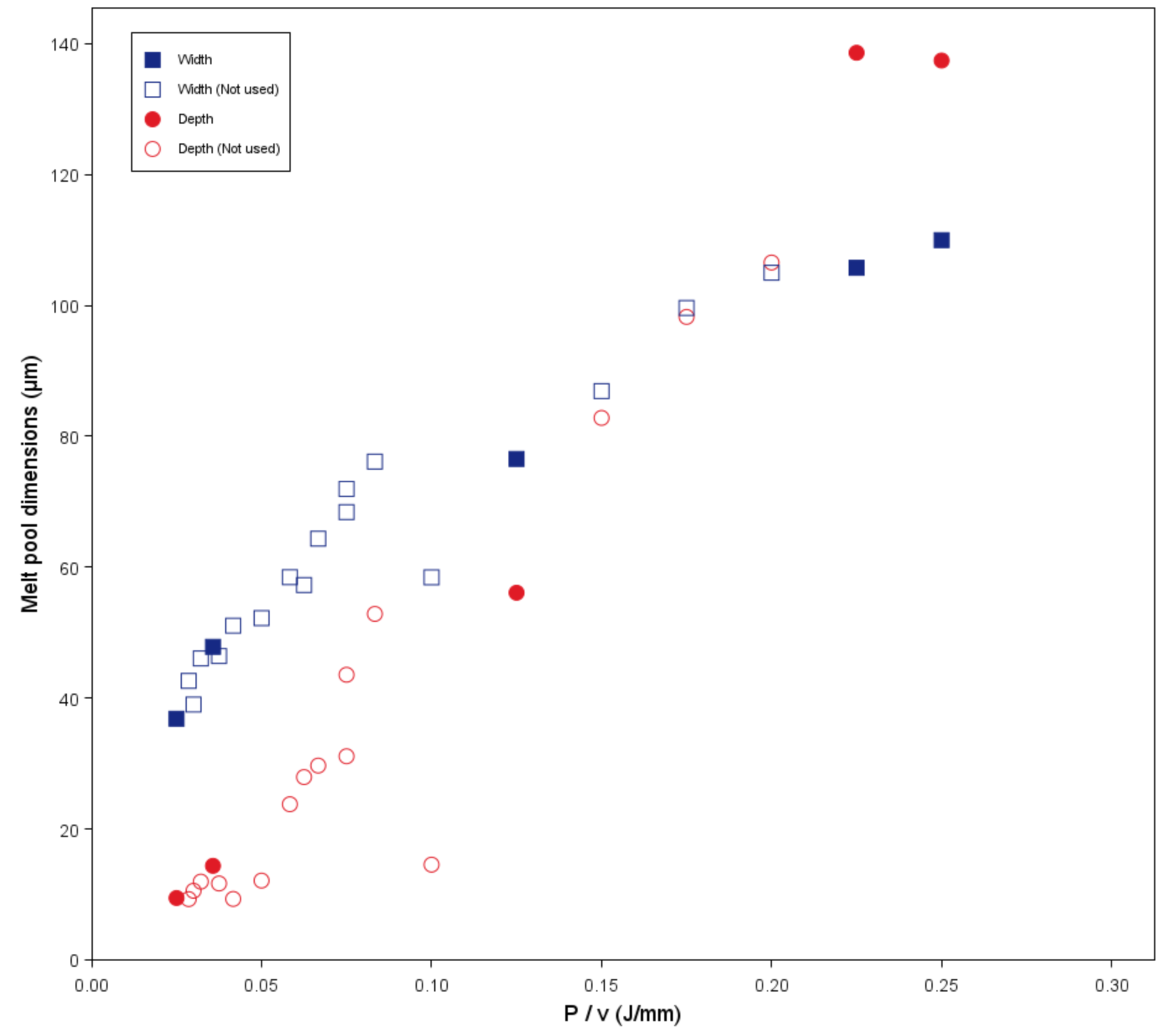
You can click or hover over any point on the Heat Source Calibration preview to display the label, which also includes the corresponding table row (i.e. Experiment) number for the point.
On the Heat Source Calibration window :
- For this calibration view, Width uses blue squares (solid color means used, hollow with same color outline means not used)
- For this calibration view, Depth uses red circles (solid color means used, hollow with same color outline means not used)
- The preview shows the energy density (P/v) on the X-axis and melt pool dimensions on the Y-axis.
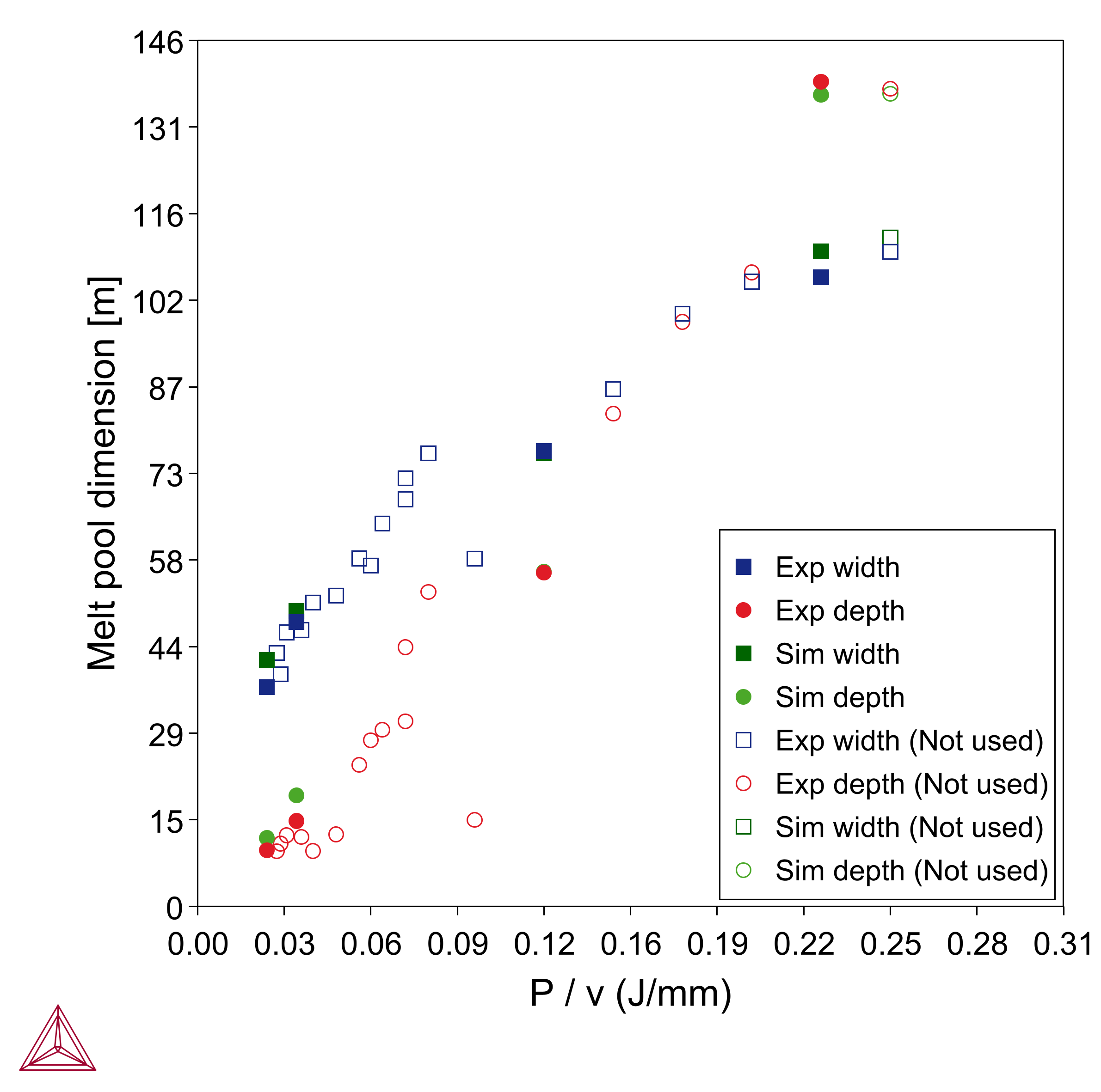
Click to select or deselect checkboxes in the table to dynamically watch the selection change on the Visualizations window. The points that are selected in this table are used in the simulation results and are later labeled Exp.Width and Exp.Depth in the Plot Renderer Configuration table (see Figure 3). Then the calculated results are added to new columns labeled Sim.Width and Sim.Depth in the data table on the Plot Renderer Configuration window (see below).
Sometimes an experiment data point is selected in the table on the AM Calculator but after running the simulation it is not available in the corresponding Plot Renderer table (i.e. it is a greyed out row). This indicates that the calibration could not be calculated for that particular data point.
Figure 1: From example AM_06a, this is the heat source calibration preview for the data imported to the AM Calculator node (renamed to AM Calibration Double Ellipsoidal). As per the legend, both "used" (solid color) and "not used" (hollow with outline color) points are included in this preview.
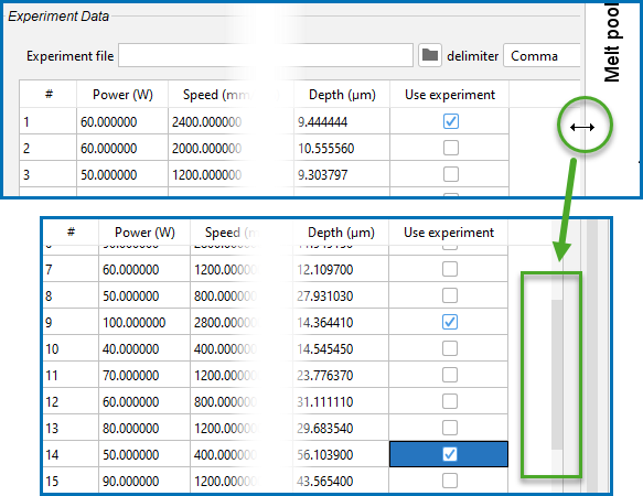
Once a set of data is imported to the table (or entered manually), expand the Configuration window to reveal the scroll bars. Then you can scroll up or down, left or right, within the table to select checkboxes for the relevant data points you want to include or exclude. This is applicable to the tables found on the AM Calculator as well as those on the Plot Renderer for the data.
Working with the Plot Renderer for Heat Source Calibrations
After the calibration is completed on the AM Calculator and the simulation run, then on the Plot Renderer Configuration window you can start to use the data.
For additional Plot Renderer settings (and other visualization options for plotting) go to AM Calculator: Plot Renderer Settings.
- Add a Plot Renderer to the AM Calculator.
- Choose an experiment point from the Heat Source Calibration list. The points in this list match the points selected in the Use column on the AM Calculator.
- Click Perform.
- Click the Heat Source Calibration tab on the Plot Renderer Configuration window to (1) view the table of data and (2) view the Heat Source Calibration Parameters and Melt Pool Dimensions tabs in the Visualizations window on the secondary level of tabs. These tabs are where you fine-tune the choice of data points: Click the checkbox for the Use column for each row (experiment #) to observe the dynamic changes on the Heat Source Calibration Parameters and Melt Pool Dimensions tabs on the Visualizations window.
On the Heat Source Calibration tab (Plot Renderer) the table includes these columns:
- The original experiment data for Power (W) and Speed (mm/s), plus the energy density P/v (J/mm).
- The original experiment data for Width and Depth, now with a prefix Exp. to indicate this is the experimental data, e.g. Exp. width (μm).
- The calculated Width and Depth points, with the prefix Sim. to indicate it is the result of the simulation, , e.g. Sim. width (μm).
Only the experiment data points selected for inclusion when setting up the AM Calculator have data in these two Sim. columns.
- The Use column has a checkbox available to include or exclude those points on the Heat Source Calibration Parameters and Melt Pool Dimensions tabs on the Visualizations window. Furthermore, if a simulation is not used in a fit, the results from that simulation are not included to generate functions for Heat Source Calibration parameters.
Only points that were originally included in the simulation can be selected or deselected from the Use column. If an experiment data point needs to be added, return to the AM Calculator, choose the point (s) to include there, and run the simulation again. Once the simulation is complete, the points are included in this table.
Figure 2: From example AM_06a, the Heat Source Calibration tab on the Plot Renderer for a double ellipsoidal heat source calibration for the double ellipsoidal heat source calculation. Here experiment from row #1 is included in the simulation as indicated by the white row and the check mark in the Use column. Rows 2-4 were not included in this simulation and are greyed out. When a checkbox is not selected, the results are also not included if you choose to export the result files.
Based on the type of heat source selected on the AM Calculator, below the Heat Source Calibration table there are additional parameters you can choose to include or exclude from the Heat Source Calibration Parameters and Melt Pool Dimensions plots.
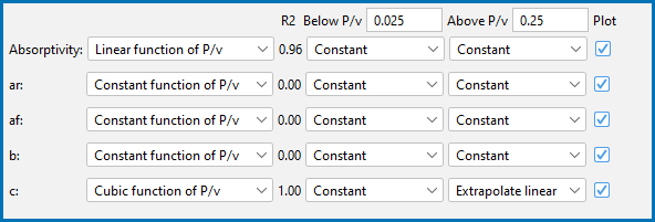
Once the selection of experiments is made in the Configuration window for the Heat Source Calibration, you can choose appropriate functions for each heat source parameter including the absorptivity. See Figure 3 for an example of the available parameters for a Double ellipsoidal Heat Source.
Figure 3: From example AM_06a, these are the available parameters for a double ellipsoidal heat source simulation. The available parameters are based on the heat source chosen on the AM Calculator during set up.
Click to select or deselect the Plot checkbox and watch the change on the Visualizations window for both the Heat Source Calibration Parameters and Melt Pool Dimensions plots. There are several options to choose from in this section that each change the plots dynamically.
The heat source parameters available to plot for each Heat Source type (i.e. Gaussian, Double ellipsoidal, or Conical) selected on the AM Calculator:
- Gaussian: Beam radius. Then based on the Absorptivity setting—Calculated (prefactor calibrated) or Constant (calibrated)—also Absorptivity prefactor plus additional options.
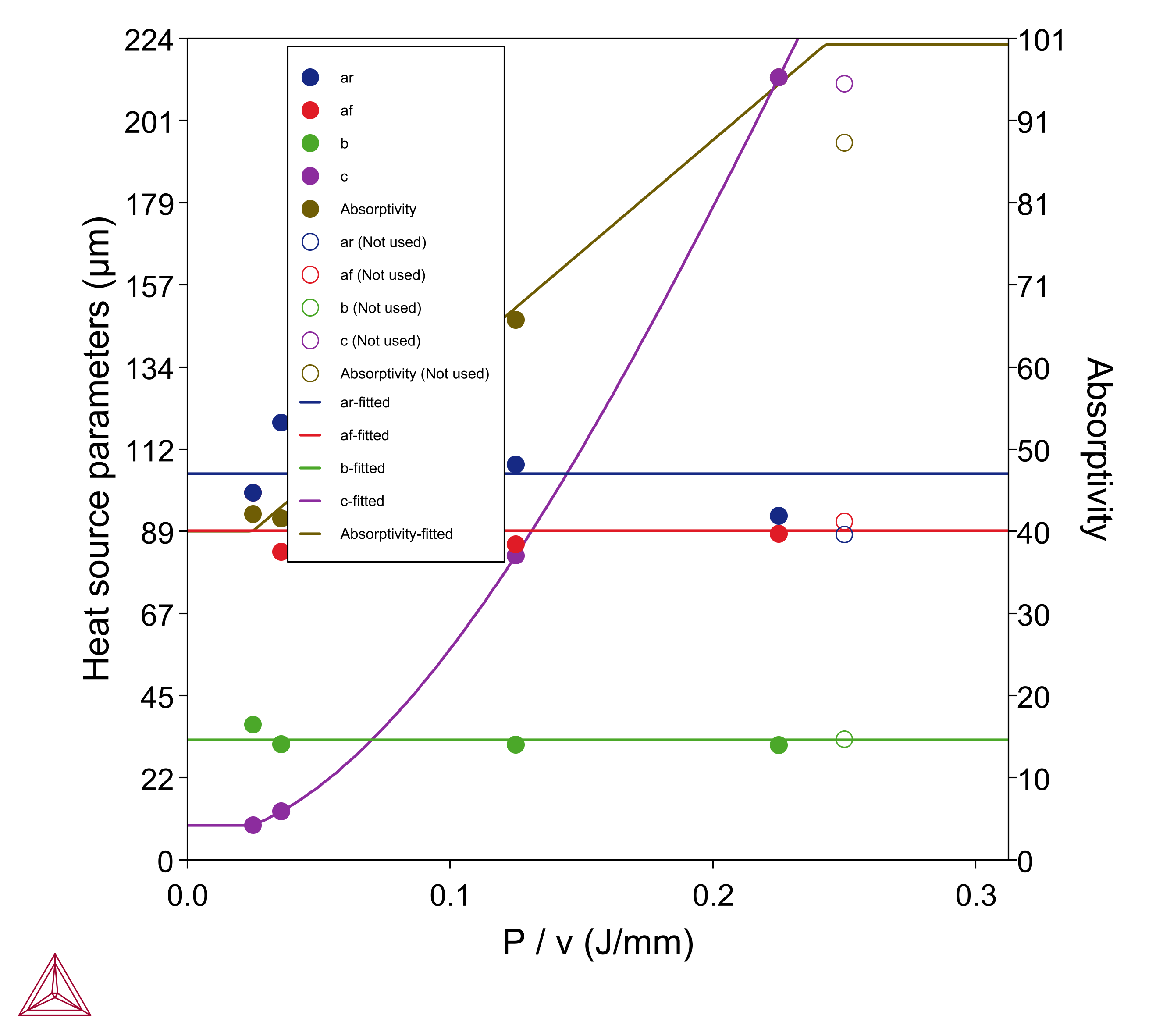
- Double ellipsoidal: Absorptivity, ar, af, b, and c
- Conical: Absorptivity, re, ri, and H.
There is more information about using these parameters in AM Calculator Heat Source Settings.
For all heat source parameters, you can also choose to select:
- A Constant function value i.e. the average value from all experiments or a function of energy density, which could also be a Linear function, Cubic function, or a Sigmoid function.
- A 2d cubic function P and v of Power (P) and Scanning speed (v).
- For extrapolating outside the range of energy density as given from the experimental data, select a Constant value, Extrapolate linear, or choose Extrapolate for extrapolation using the same function as chosen for interpolation.
- Set the range of energy density to interpolate the heat source parameters by entering the appropriate values in the Below P/v and Above P/v fields.
There are R2 values (the coefficient of determination) included that say how well the selected function fits the data. R2 ranges from zero to one, where 1 is a perfect match. E.g. A linear function between two points.
Once all the parameter adjustments are made, you can also retain this information for future reuse (click Save As or Save). You can also Rename or Delete these from the list as needed.
The name of the file defaults to using the Heat Source type + the material type. For example, Double ellipsoidal - 316L, or Gaussian - 316L.
Visualizations Window
A Heat Source Calibration Parameters plot shows the calibrated heat source parameters as a function of energy density (P/v) (unit J/mm). From the Plot Renderer Configuration window, you can also continue to select which experiments to be used to fit the calibration.
Figure 4: From example AM_06a, the Heat Source Calibration Parameters plot for the double ellipsoidal calibration.
For instance, you can deselect the points that seem to be outliers or where the error bar in experimental data is large.
The selection is done via the checkboxes available in the Use column.
A Melt Pool Dimensions plot shows melt pool size, both from experiments and simulations, as a function of energy density (P/v). This plot can be used to compare the results from the experiments and optimization simulations.
Use a 3D Plot to visualize all the experiments for which the calibration is performed. To show the 3D plot for a certain experiment, select the corresponding experiment from the Heat Source Calibration Experiments menu. The configuration in the 3D Plot works in the same way as for a single point steady-state calculation.
For Plot Over Line, plot the data along a line for the selected experiment. To show the plot over line for a specific experiment, select the corresponding experiment from the Heat Source Calibration Experiments menu. The configuration in the Plot Over Line works in the same way as for a single point steady-state calculation.

