AM_06a: Calibrating a Heat Source for a 316L Steel
This example demonstrates the calibration of the heat source using the Gaussian as well as Double ellipsoidal heat sources. In this example, experimental data is taken from Hu. et al. [2019Hu] where the authors performed single-track experiments using the selective laser melting (SLM) process on 316L stainless steel for varying processing conditions. The power ranges from 50 W to 100 W while the scanning speed varies from 400 mm/s to 2800 mm/s. The data imported from [2019Hu], consisting of 21 experimental points, is saved in the project file.
Also see the companion example, AM_06b: Using the Calibrated Heat Source for a 316L Steel.
Material Properties
- SS316L: Fe-17.0Cr-12.0Ni-2.5Mo-0.03C Mass percent
- Database: TCFE13
- The material properties are precalculated, and stored as a built-in material library with the Additive Manufacturing (AM) Module.
AM Calculator Configuration Settings
The AM_06a example contains two AM Calculators, which are renamed to AM Calibration Gaussian and AM Calibration Double Ellipsoidal.
- AM Calibration Gaussian uses a Gaussian Heat Source with the keyhole model.
- AM Calibration Double Ellipsoidal uses a Double ellipsoidal Heat Source.
- The heat source parameters for both heat sources are calibrated for the given experimental data.
- For both AM Calculators, the Base plate temperature and the Ambient temperature use a value of 353 K and the Layer thickness is 10 μm. The rest of the Configuration settings keep the original defaults.
For AM Calibration Gaussian, all of the 21 experimental points that are imported to the Experiment Data table are selected to be used in the calibration. This is because, for the Gaussian heat source with the keyhole model, one wants to obtain a single constant value for beam radius as well as absorptivity to correctly predict the melt pool size for a range of power and scanning speed. It is also in order to obtain the best possible value it is good to include as many experiments as you can to calibrate the heat source parameters.
For this AM Calculator, other settings include:
- Constant (calibrated), which means the absorptivity is not a function of temperature or angle, and a constant value is calibrated for each experiment.
- The Beam radius is set to Calibrated, which means that both beam radius and absorptivity are calibrated.
- Calibrate for is set to Width and depth, which means that the experimental values for both width and depth are used for calibration.
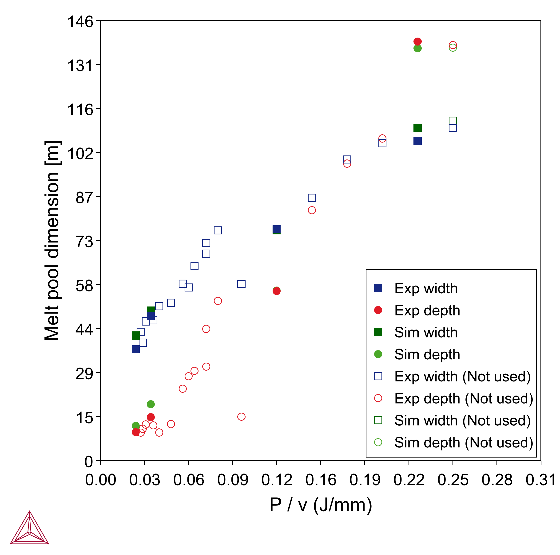
For AM Calibration Double Ellipsoidal, only five (5) experiment points are selected to perform the calibration. Two experiments are selected from the lower energy density, two from the higher energy density, and then one experiment is selected in the middle region of the two extremes.
Visualizations
Open the example project file to review the node setup on the Project window and the associated settings on the Configuration window for each node. For some types of projects, you can also adjust settings on the Plot Renderer Configuration window to preview results before performing the simulation. Click Perform Tree to generate plots and tables to see the results on the Visualizations window.
When you run (Perform) this example, it can take about an hour to complete the calculations.
There is a variety of information shown in the Visualizations window that can be viewed during configuration and after performing the calculation(s).
See Visualizing Heat Source Calibrations for an extended overview of what is available and how to navigate the many options for visualizing the heat source calibration data.
Calibrated Functions
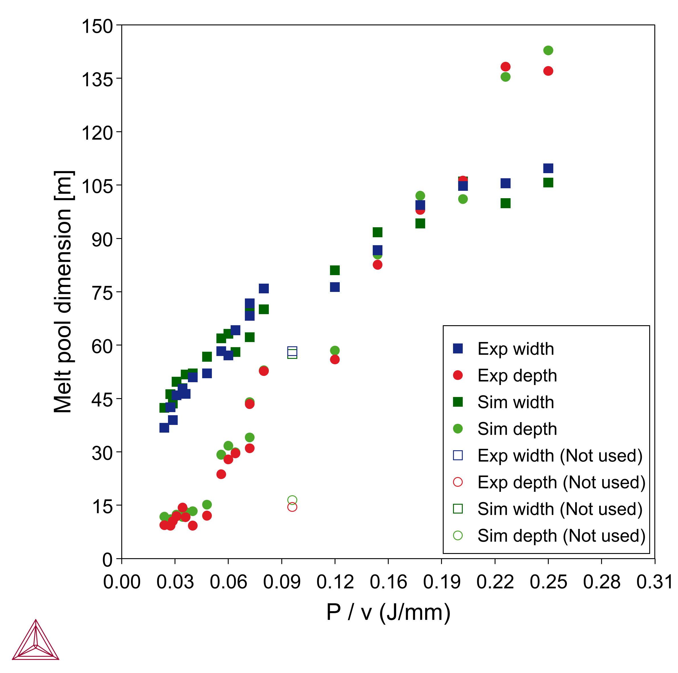
For AM Calibration Gaussian, a comparison of the melt pool dimensions from the experiments and calibration simulation is shown in Figure 1.
Figure 1: A comparison of melt pool dimension for Gaussian heat source calibration. The "Not used" points shown in the legend are because a checkbox is not selected in the 'Use' column for row 10 on the Plot Renderer Configuration window.
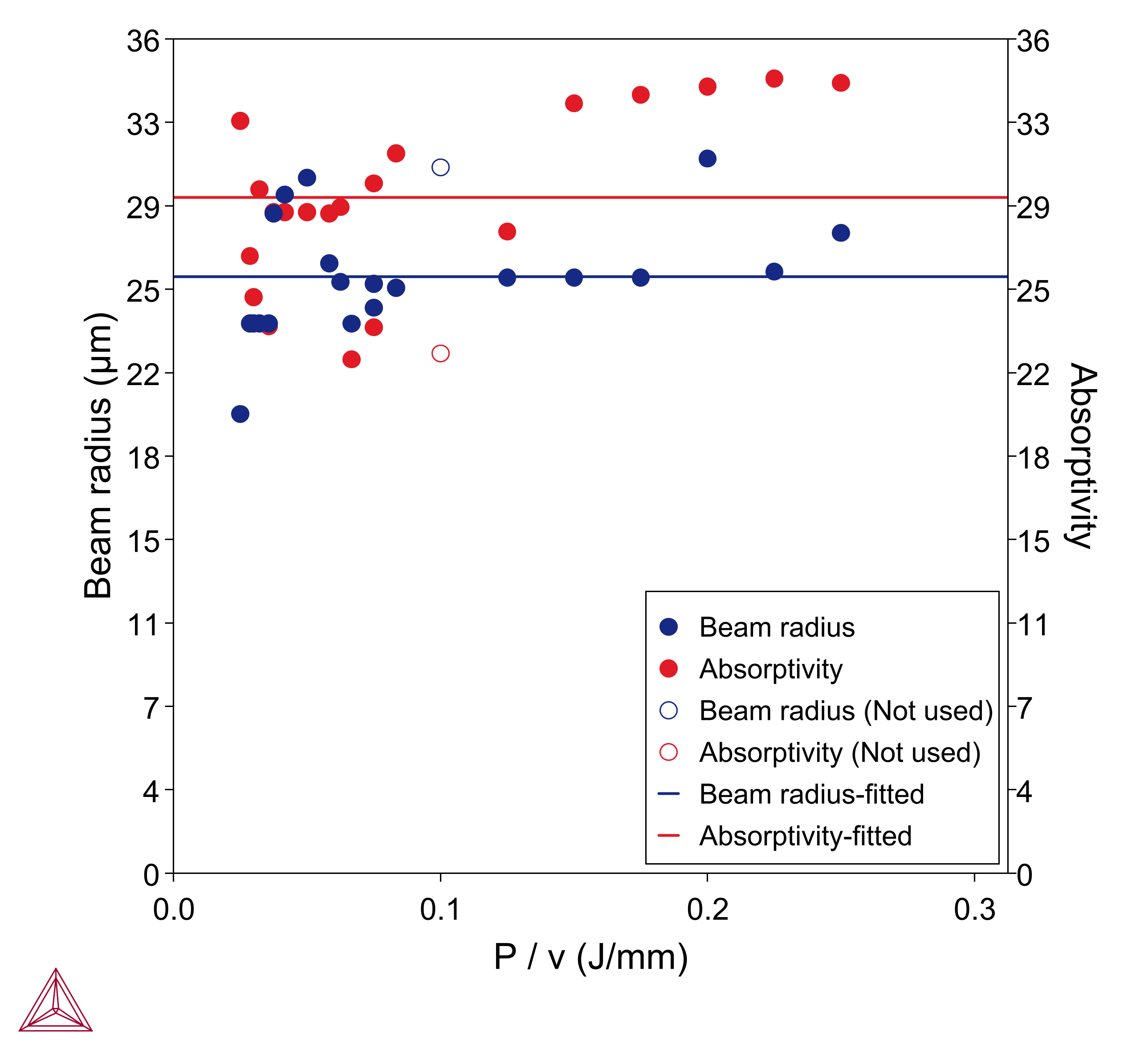
The resulting calibrated heat source parameters for AM Calibration Gaussian, are shown in Figure 2.
In order to obtain the expressions for Absorptivity and Beam radius, one of the experiments (Experiment # 10) is not included. This is because Experiment # 10 is an outlier and you can see that the values for Exp width and Exp depth (hollow square) then the Sim width and Sim depth (hollow circle) are excluded in Figure 1.
For both Absorptivity and Beam radius the Constant function of P/v is chosen to be saved as a calibrated heat source. Absorptivity of the material at the printing conditions is usually unknown in these experiments which is why it is regarded as a fitting parameter. Beam radius, on the other hand, is most often known, but does not match the definition of beam radius in the Gaussian heat source model used in the simulation, which is why a different value is obtained as compared to the one used in the experiment.
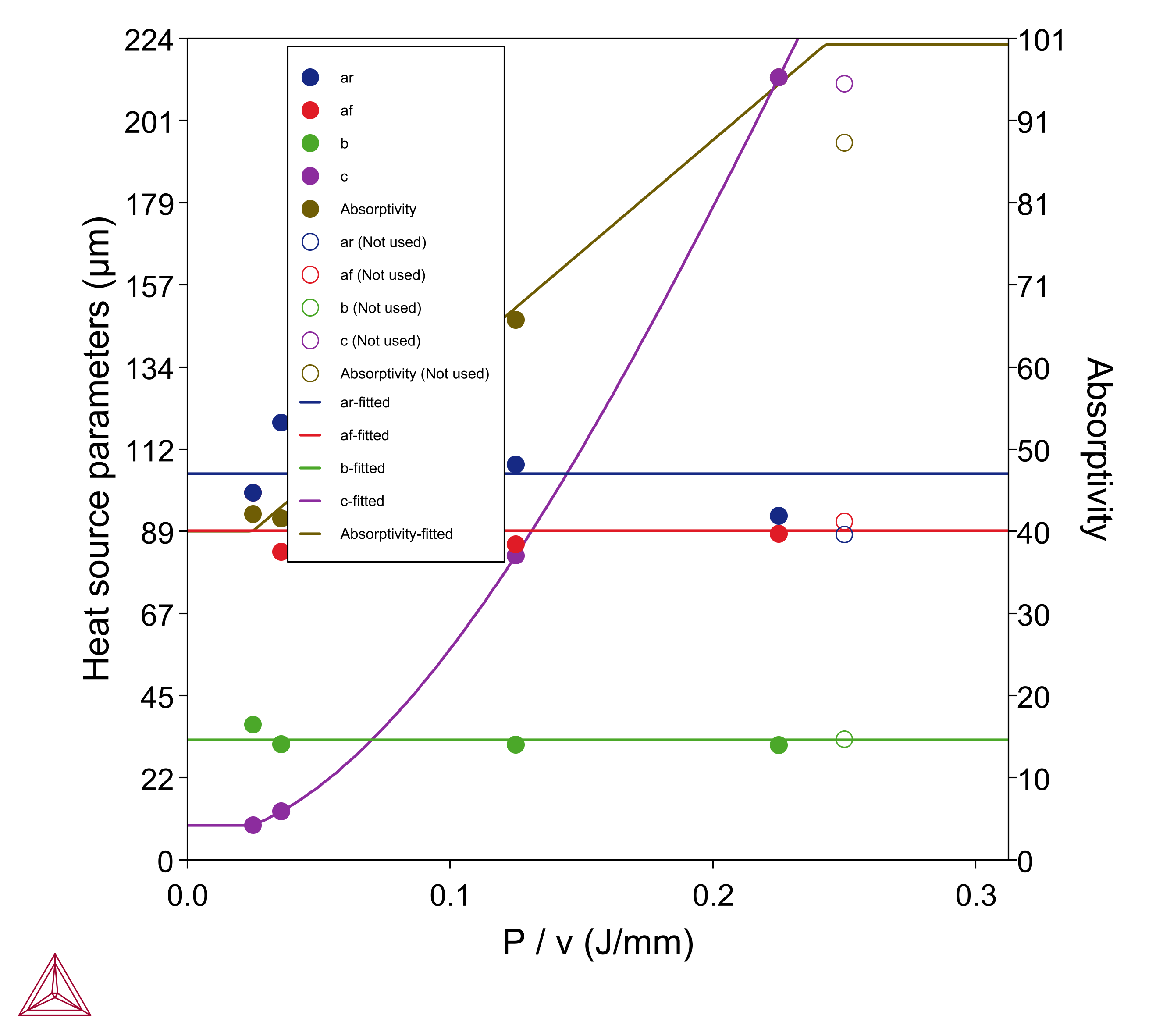
While selecting the functions for heat source parameters for double ellipsoidal, it was seen that ar, af, and b remained almost unchanged for all the experiments. Therefore the Constant function of P/v for ar, af, and b is used. For Absorptivity, a Linear function of P/v gave the best R2 value while for c a Cubic function of P/v gave the best R2 value. One of the experiments (experiment # 21) was excluded (i.e. the checkbox is deselected) to get a suitable curve for all functions.
Reference
[2019Hu] Z. Hu, B. Nagarajan, X. Song, R. Huang, W. Zhai, J. Wei, Formation of SS316L Single Tracks in Micro Selective Laser Melting: Surface, Geometry, and Defects. Adv. Mater. Sci. Eng. 2019, Article ID 9451406, 1–9 (2019).
Other Resources
Read more about the Additive Manufacturing (AM) Module on our website including the details about database compatibility or to watch an introductory webinar. You can also use the Getting Started Guide to learn about the key features available.
Many of our Graphical Mode examples have video tutorials, which you can access in a variety of ways. When in Thermo‑Calc, from the menu select Help → Video Tutorials, or from the main My Project window, click Video Tutorials. Alternately, you can go to the website or our YouTube channel.


