PM_G_02: Coarsening and Interfacial Energy
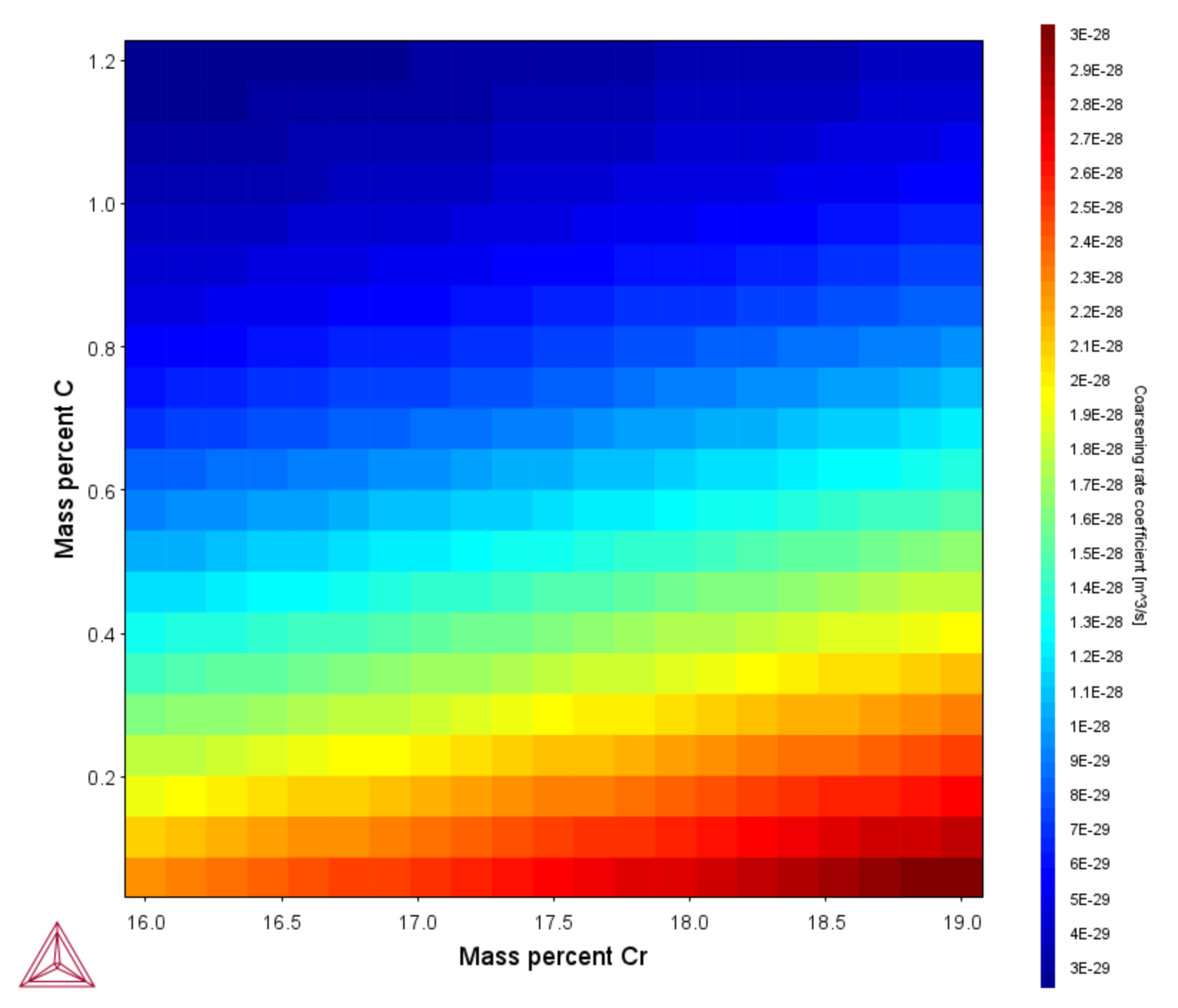
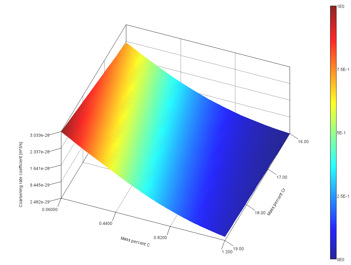
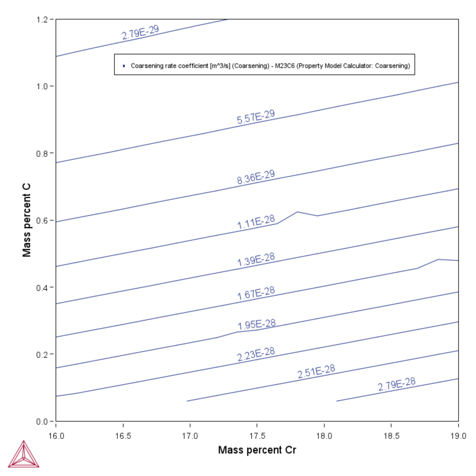
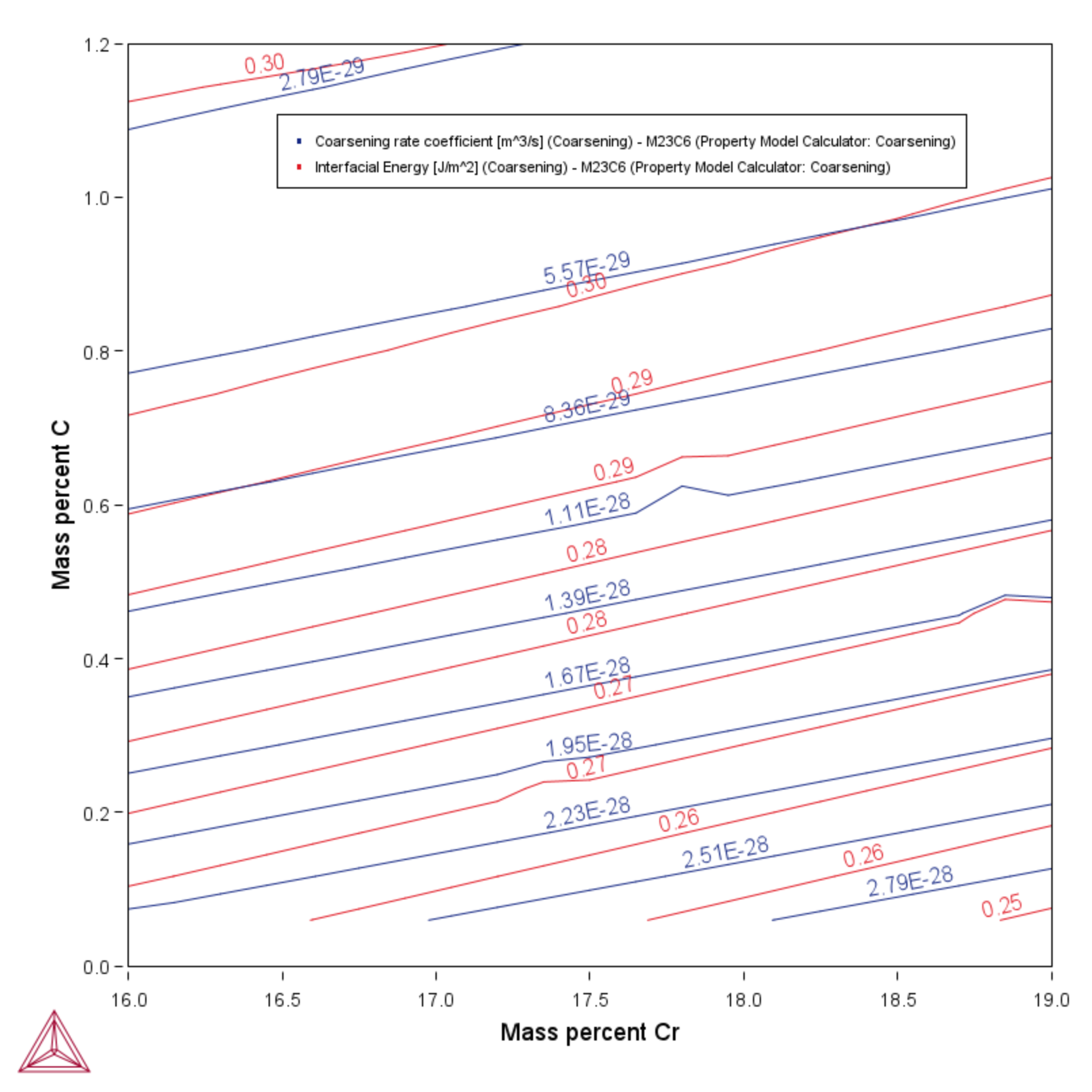
The example uses the Property Model Calculator and both thermodynamic (FEDEMO) and kinetic (MFEDEMO) demonstration steel databases. Using a Grid Calculation Type it produces these plot types: a Heat map, a Contour plot and an overlaid plot combining a cross plot with a contour plot (where both the interfacial energy and coarsening rate is shown). It also creates a diagram to show the phase fractions vs time and a 3D Plot type comparing the coarsening rate coefficient.
Coarsening Property Model Settings
- Folder: Property Models → General
- File name: PM_G_02_Coarsening_and_Interfacial_energy.tcu
Visualizations
This example is included as a Property Model tutorial on our website and as part of the Property Model Calculator playlist on our YouTube channel.
Open the example project file to review the node setup on the Project window and the associated settings on the Configuration window for each node. For some types of projects, you can also adjust settings on the Plot Renderer Configuration window to preview results before performing the simulation. Click Perform Tree to generate plots and tables to see the results on the Visualizations window.
Figure 1: Uses a Property Model Calculator with a Grid Calculation type to plot the coarsening rate coefficient as a Heat map.
Figure 2: Uses a Property Model Calculator with a Grid Calculation type to plot the coarsening rate coefficient as a 3D plot.
When in the Thermo-Calc help (press F1), go to Rotating 3D Plots to watch a short video showing you how to rotate this plot in the Visualizations window.
Figure 3: Uses a Property Model Calculator with a Grid Calculation type to plot the coarsening rate coefficient as a Contour plot.
