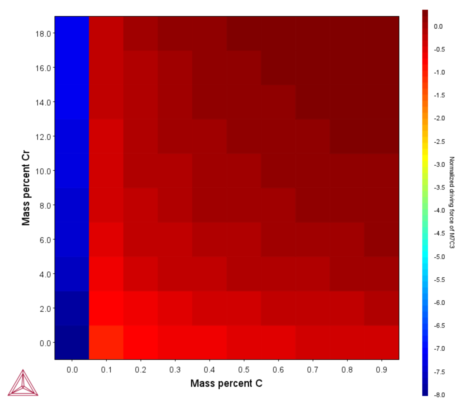
T_09: Carbide Driving Force Heat Map
This is an example of using Grid calculations to plot the driving force for a carbide as a function of two composition variables. With the Grid Calculation Type, a 2D grid is generated from the two calculation axes. After the calculation is done, an equilibrium is calculated in each grid point. A
In the Plot Renderer settings window, click Show more and Show less to toggle between viewing all or some of the available settings.
- Folder: Thermo‑Calc
- File name: T_09_Heat_map_of_carbide_driving_force.tcu
Visualizations
This example is included as a tutorial on our website and as part of the Graphical Mode Examples playlist on our YouTube channel.
Open the example project file to review the node setup on the Project window and the associated settings on the Configuration window for each node. For some types of projects, you can also adjust settings on the Plot Renderer Configuration window to preview results before performing the simulation. Click Perform Tree to generate plots and tables to see the results on the Visualizations window.
