P_16 Isothermal Coarsening and a 3D to 2D Stereological Conversion

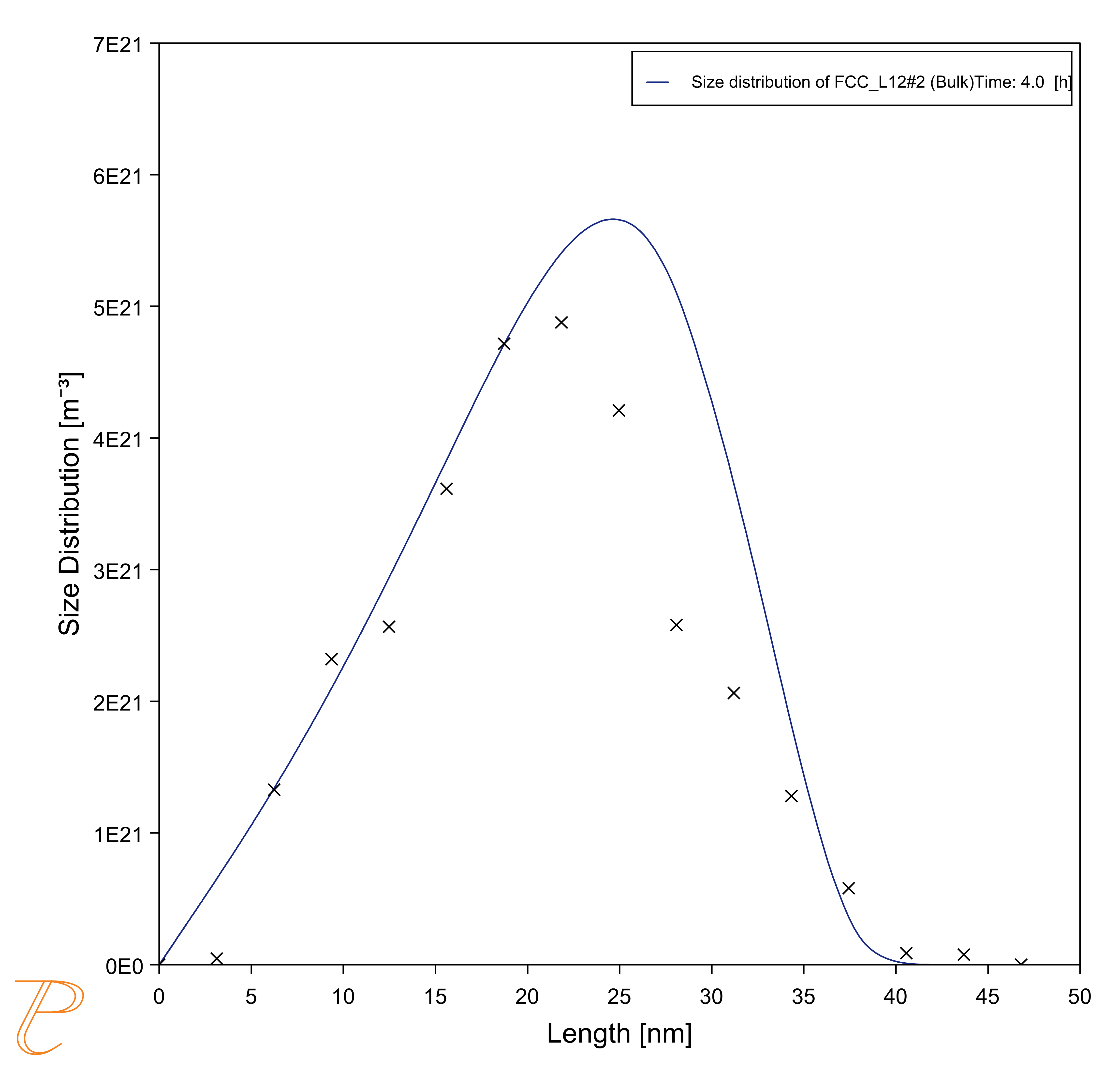
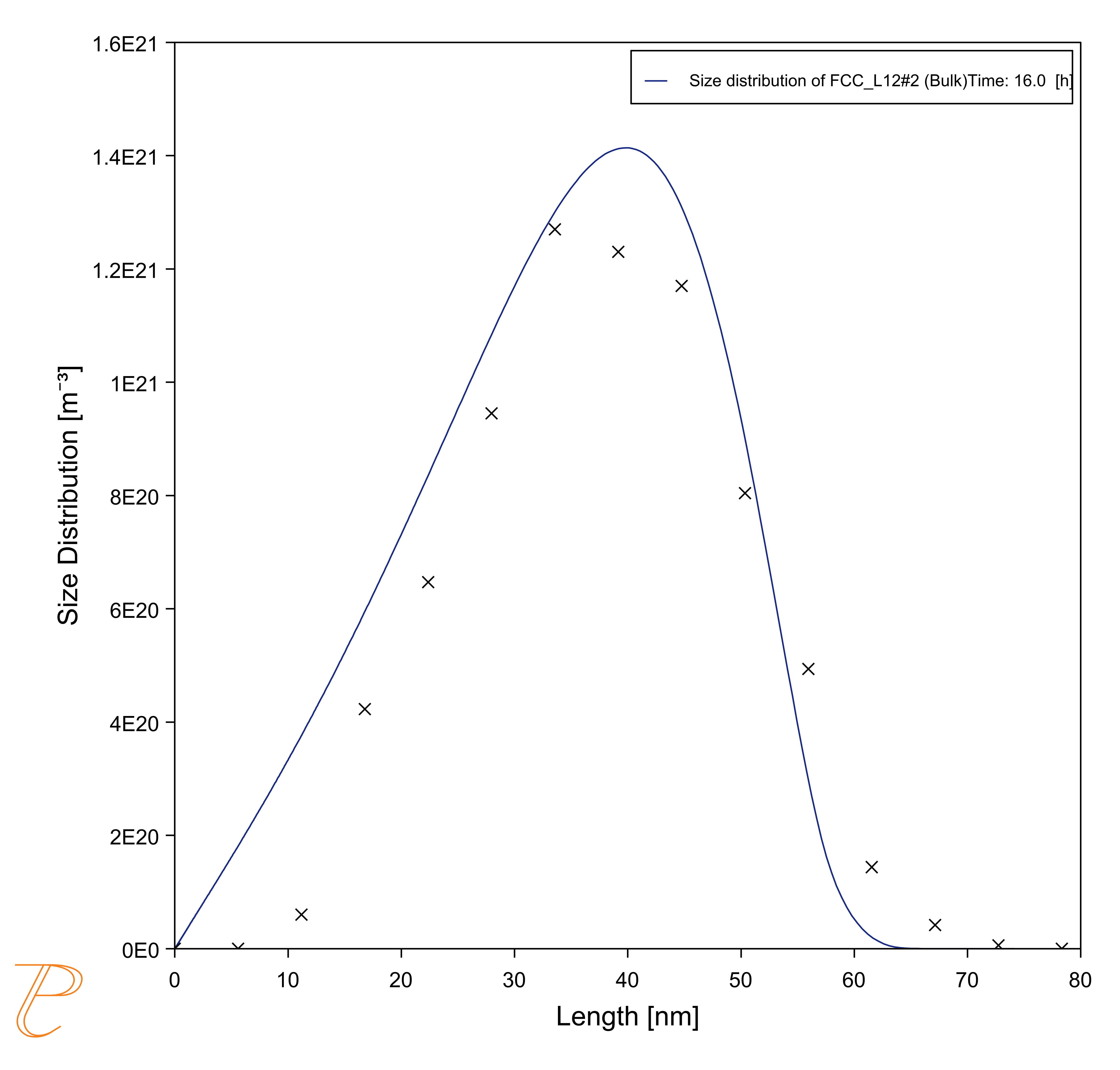
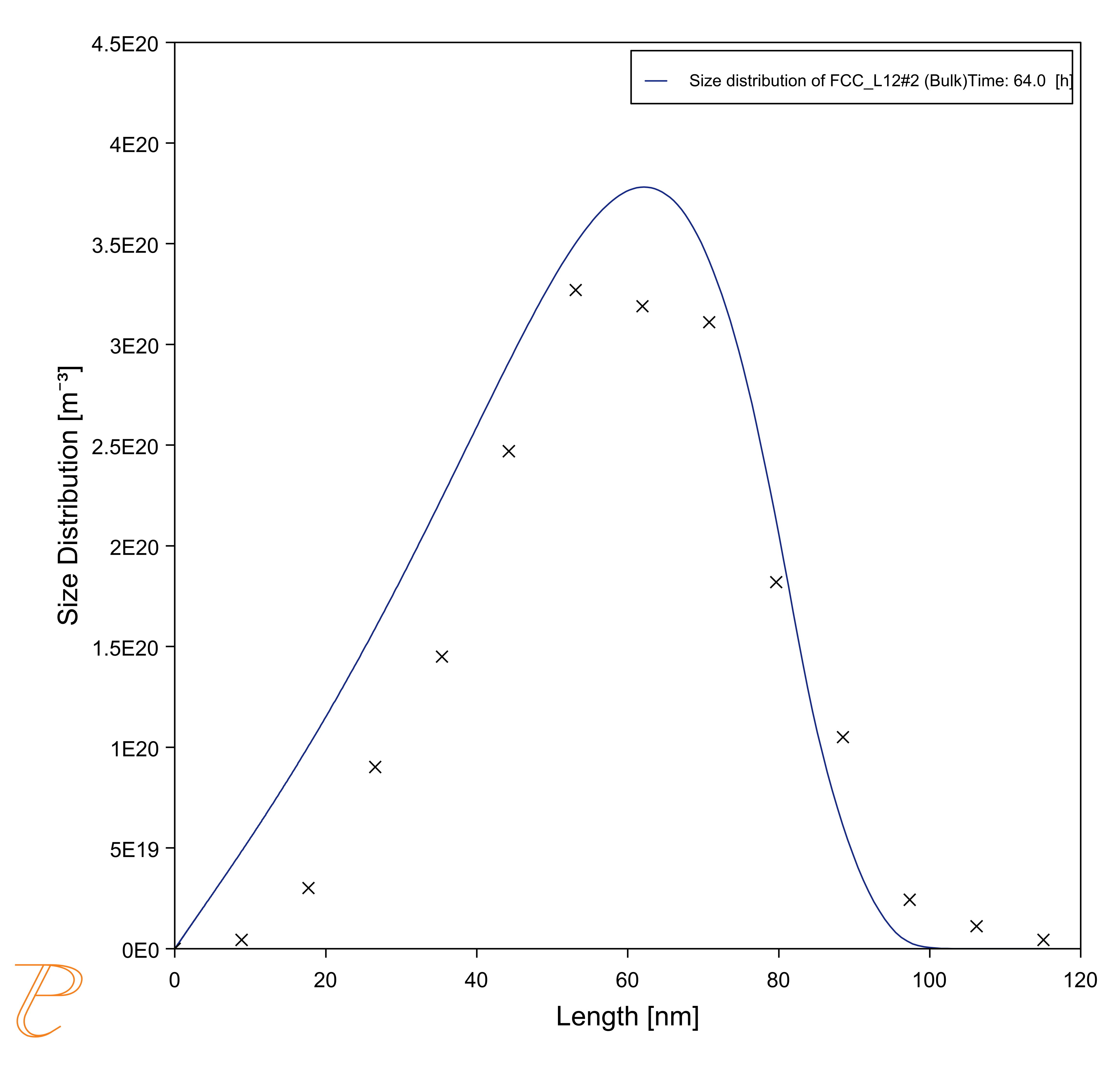
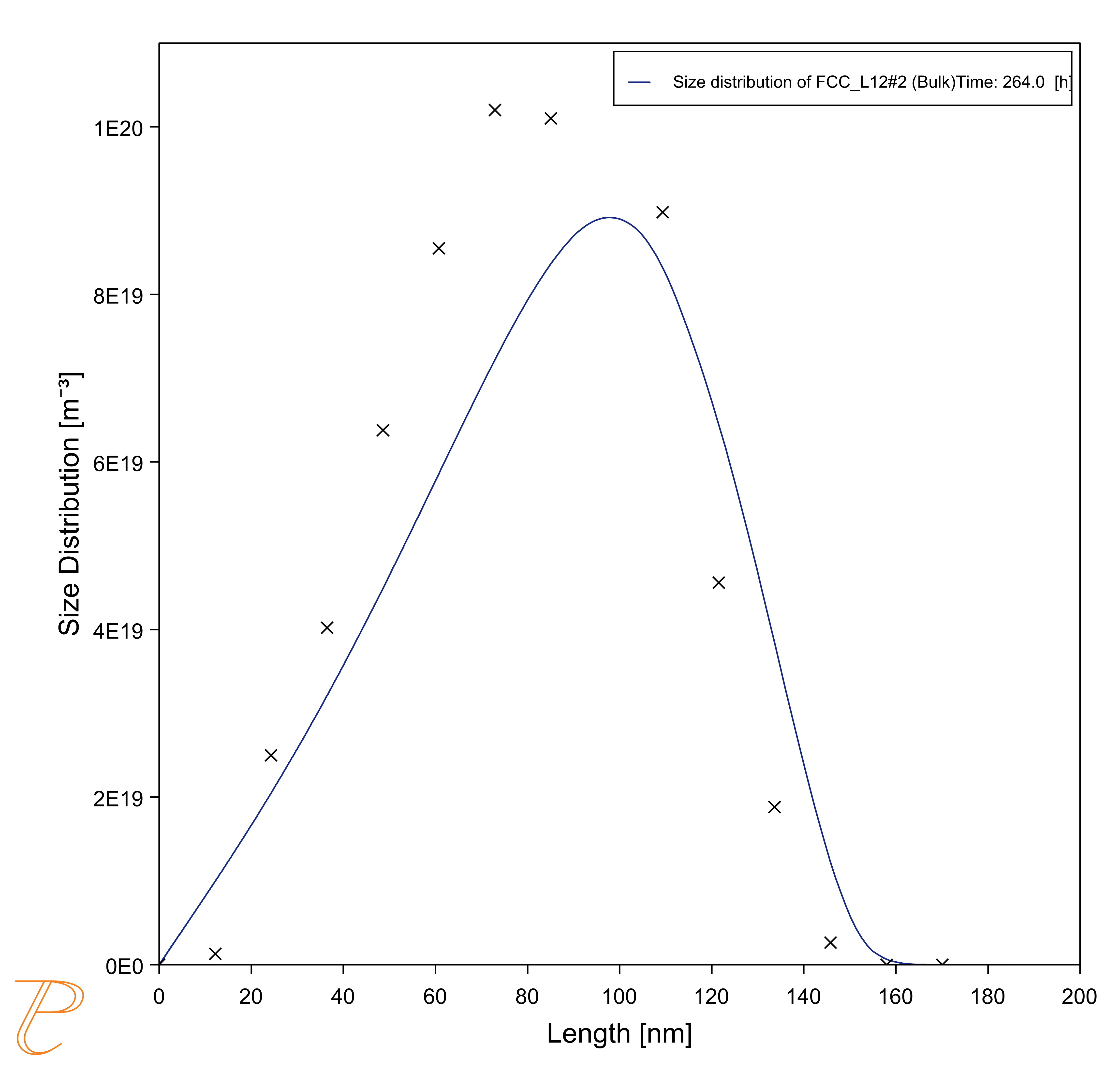
This example demonstrates the use of the 3D → 2D stereological conversion functionality to compare Precipitation Module (TC-PRISMA) predictions with experimental data obtained from Scanning Electron Micrographs (SEM).

The 3D → 2D setting is available on a Plot or Table Renderer that is a successor to the Precipitation Calculator, and when certain axis variables are selected for a spherical morphology.

For more background information, see the theory described in Stereology.

The isothermal coarsening kinetics of γ' precipitates in a Ni-Al-Cr alloy is modeled. The experimental data is from [2008Sud], which investigates isothermal coarsening kinetics at a temperature of 873 K for up to 264 h.

It is assumed that there are no precipitates in solution at the beginning of the isothermal heat treatment.

Example Settings

The example also includes an Equilibrium Calculator and Table Renderer to first confirm the stability of the precipitate phase for this system (FCC_L12#2), then determine particle composition at 1073 K, and this information is used with the Precipitation Calculator set up.

System (System Definer)
Database package	Demo: Nickel-based superalloys (NIDEMO and MNIDEMO)
Elements	Ni, Al, Cr
Conditions (Precipitation Calculator)
Composition	Ni-10l-8.5Cr Mole percent
Matrix Phase	FCC_L12 Click Show Details and for the Mobility adjustment enter 0.5 for the Prefactor. All other defaults are kept.
Precipitate Phase	FCC_L12#2 Click Show Details and adjust the default settings as indicated: Interfacial energy: Select User-defined and enter 0.01 J/m2.
Calculation Type (Precipitation Calculator)
Calculation Type	Isothermal
Temperature	1073 Kelvin
Simulation time	300 h
Datasets (Experimental File Reader)
2008 Sudbrack et al	Data sets are included with this example and are imported using the Experimental File Reader activity. There are 2D size distributions comparing results after a total of 16 h aging, 64 h aging, and 264 h of aging, and a comparison of the experimental and predicted 2D mean radius versus time.

Visualizations

Many of our Graphical Mode examples have video tutorials, which you can access in a variety of ways. When in Thermo‑Calc, from the menu select Help → Video Tutorials, or from the main My Project window, click Video Tutorials. Alternately, you can go to the website or our YouTube channel.

Open the example project file to review the node setup on the Project window and the associated settings on the Configuration window for each node. For some types of projects, you can also adjust settings on the Plot Renderer Configuration window to preview results before performing the simulation. Click Perform Tree to generate plots and tables to see the results on the Visualizations window.

There is a variety of information shown in the Visualizations window that can be viewed during configuration and after performing the calculation.

• Thermal Profile: When setting up a calculator on a Configuration window for Isothermal or Non-isothermal Calculation Types, you can preview the profile and adjust settings as needed. When you click a calculator node in the Project window, the matching name of the node is on the tab(s) displayed in the Visualizations window.

  For TTT Diagram and CCT Diagram calculations there is nothing shown for the Precipitation Calculator tab in the Visualizations window as there is no Thermal Profile to be defined.

• Plot or Table results: After completing the set up and performing the calculation, to view the matching name of the node on tab(s) in the Visualizations window, either click a Plot Renderer or Table Renderer node in the Project window or click the tabs individually in the Visualizations window.

For this Isothermal example, its Thermal Profile is also displayed in the Visualizations window showing the constant temperature entered for this calculation type. The tab names match the node names in the Project window.

Reference

[2008Sud] C. K. Sudbrack, T. D. Ziebell, R. D. Noebe, D. N. Seidman, Effects of a tungsten addition on the morphological evolution, spatial correlations and temporal evolution of a model Ni–Al–Cr superalloy. Acta Mater. 56, 448–463 (2008).