AM_02: Transient and Steady-state Simulations of a Single Track

The following example is part of a series showing some of the features of the Additive Manufacturing (AM) Module and the AM Calculator. This example builds on the work done by Grange et al. [2021Gra] and is similar to example AM_01. The difference however is that in this example a single track simulation is performed using Transient with heat source from Steady-state model instead of the Transient model.

The Transient with heat source from Steady-state model exploits the assumption that the melt pool size and temperature distribution reaches a steady-state almost instantly and thus first solves for a Steady-state case with the given process parameters. The result from the Steady-state in the form of temperature distribution in the melt pool is then mapped as a heat source in the transient simulation. This novel approach is much faster and efficient than the approach used in example AM_01 where the heat equation is solved in the entire 3D domain.

Material Properties

These properties are the same for both AM_01 and AM_02 [2021Gra].

Inconel 738LC: Ni-15.8 Cr-8.6 Co-2.7 W-3.3 Ti-3.6 Al-1.8 Ta-1.8 Mo-0.04 Fe-0.8 Nb-0.002 Mn-0.1 C Mass percent.
Database: TCNI12
The material property was pre-calculated, and stored as a built-in material library of the Additive Manufacturing (AM) Module.

Model Configuration

The transient model solves for the heat equation in the entire 3D domain, including the melt pool, and is therefore, computationally expensive to solve. The fluid flow inside the melt pool due to the Marangoni effect is not included in this example. The double ellipsoidal, or the so-called Goldak heat source model, is used to predict melt pool size and temperature distribution during single track scanning. The parameters for the double ellipsoidal heat source are computed using optimization in a steady-state case for the given process parameters (power and scanning speed) and the melt pool size reported in the paper by Grange et al. [2021Gra]. The resulting parameters are shown in Figure 1.

Figure 1: Optimized heat source parameters entered on the AM Calculator for the experiment given in Grange et al. [2021Gra] with power = 230 W and scanning speed = 960 mm/s.

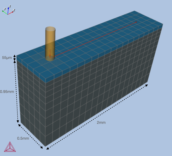
The geometry for a transient simulation, as given in the paper by Grange et al. [2021Gra], is shown in Figure 2. The base plate is 2 mm in length, 0.5 mm in width, and with a thickness of 0.95 mm. A layer of powder with a thickness of 55 μm is deposited on the solid substrate. The powder layer, however, has the same material properties as the solid substrate. The laser beam with a power of 230 W develops linear scanning with constant velocity 960 mm/s. The trajectory evolves from initial position (x, y) = (0.25, 0.25) mm to final position (1.75, 0.25) mm on the top surface.

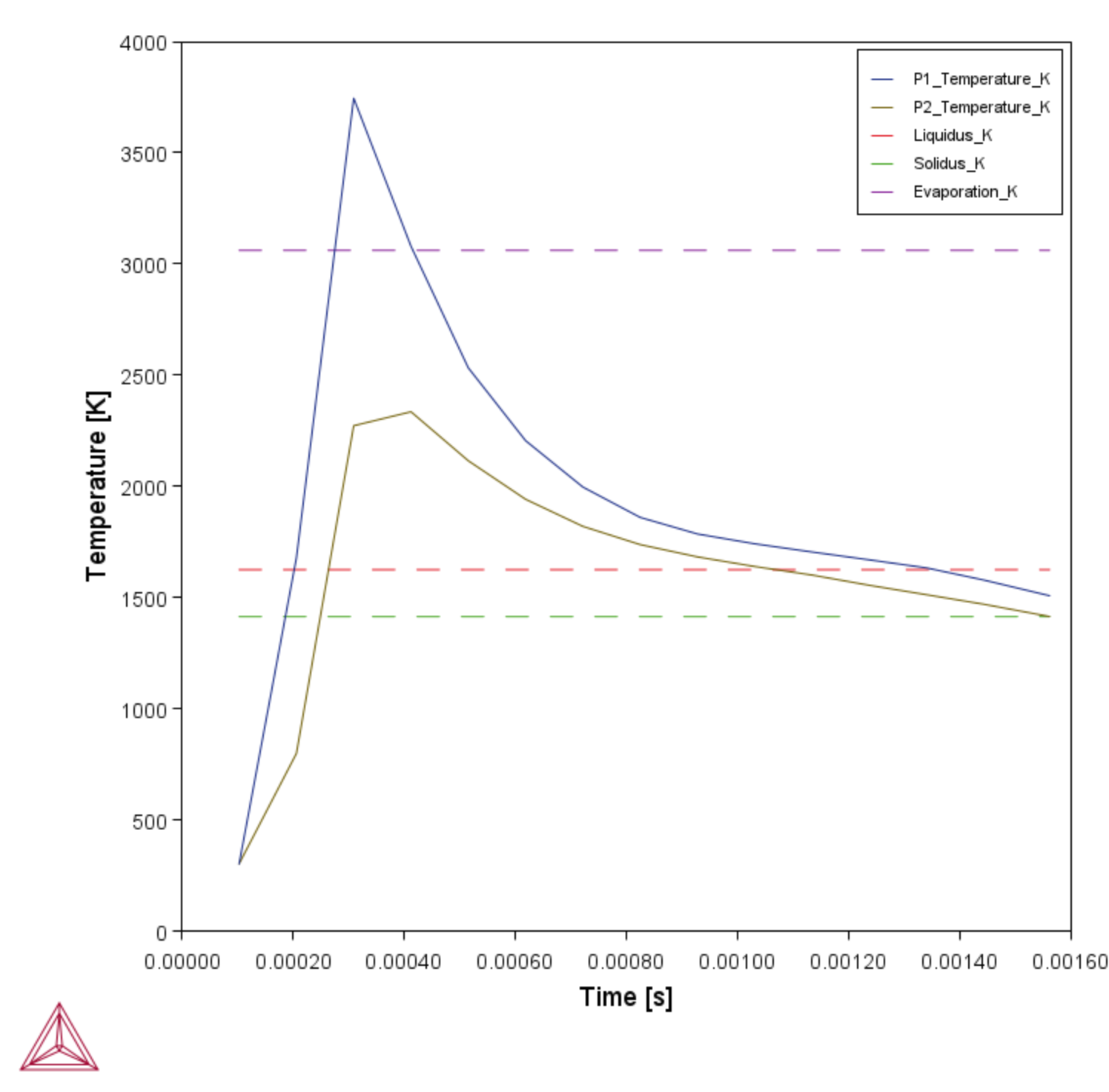
The geometry used for the examples AM_01 and AM_02.

Figure 2: The geometry used for the Additive Manufacturing (AM) Module examples AM_01 and AM_02.

Two probes monitor the temporal evolution of temperature at positions shown in Figure 3. The results can be presented by tabulated data or as 2D graph plots.

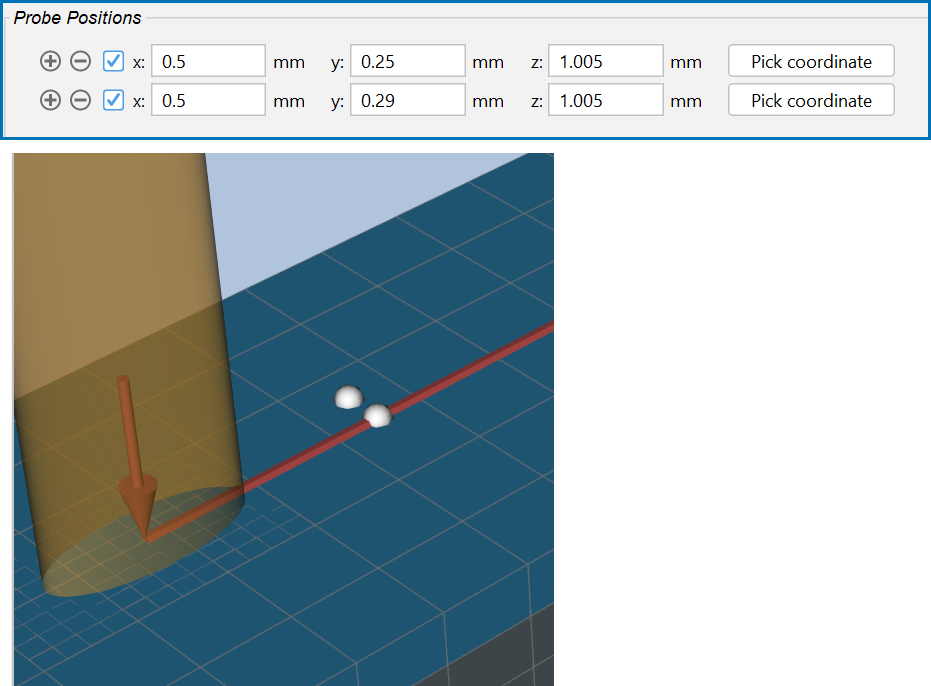
Probe positions for Probes P1 and P2, where P1 is placed exactly on the scanning track while P2 is placed at a distance of 0.04 mm from the track, as shown in a close up of the probes on the Visualizations window.

Figure 3: Probe positions for Probes P1 and P2, where P1 is placed exactly on the scanning track while P2 is placed at a distance of 0.04 mm from the track, as shown in a close up of the probes on the Visualizations window.

Visualizations

Open the example project file to review the node setup on the Project window and the associated settings on the Configuration window for each node. For some types of projects, you can also adjust settings on the Plot Renderer Configuration window to preview results before performing the simulation. Click Perform Tree to generate plots and tables to see the results on the Visualizations window.

There is a variety of information shown in the Visualizations window that can be viewed during configuration and after performing the calculation(s).

Geometry: View the geometry and adjust parameters visually by changing inputs on the Configuration window.
Melt pool and other dynamically changing features can also be visualized and changed.
Plot results: After completing the set up and performing the calculation, to view the matching name of the node on tab(s) in the Visualizations window, click a Plot Renderer node in the Project window or click the tabs individually in the Visualizations window.

With the example open and after it is run, the following is a summary of what is visible on the Visualizationswindow.

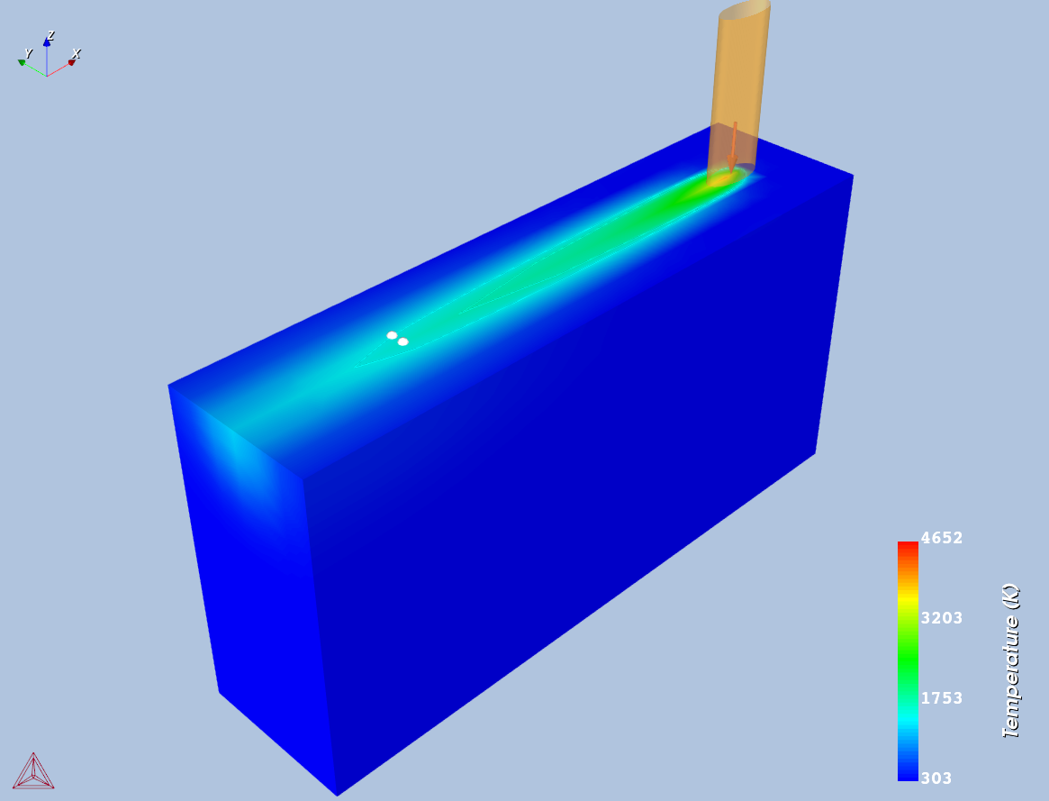
The figure below shows the surface plot of temperature distribution after the single track scanning is completed. The temperature profile is qualitatively similar to the one in example AM_01, however the maximum temperature is slightly lower in example AM_02. This could be due to selection of a coarse mesh in both examples which sometimes could affect the maximum temperature.

Figure 4: Surface plot of temperature distribution after the single track scan is completed. Probes P1 and P2 can also be seen on the top surface.

The melt pool dimensions for AM_02 are given in the following table, which are very similar to the melt pool dimensions obtained in example AM_01.

Melt Pool Dimension	Size (mm)
Width	0.127
Depth	0.129
Length	1.12

A qualitative comparison between AM_01 and AM_02 can also be made by looking at probe plots. The probe plot for AM_02 is given in Figure 5.

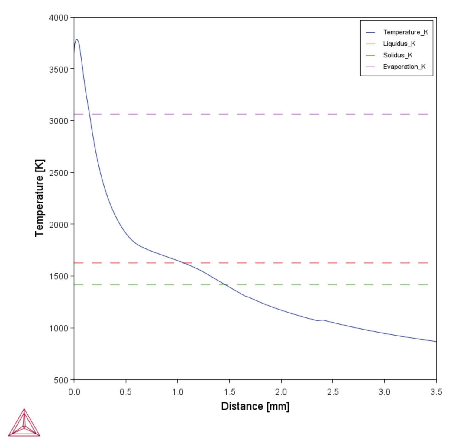
Figure 5: 2D probe plot showing temperature evolution as a function of time at probes P1 and P2.

Despite the fact that maximum temperature is higher in AM_01, the temperature profile in the tail of the melt pool and close to the melt pool is very similar. This can also be concluded by comparing plot over lines for the two examples, where the plot over line for AM_02 is given in Figure 6.

Figure 6: 2D plot over line showing temperature in the tail of the melt pool as a function of distance plotted along the scanning track.

Reference

[2021Gra] D. Grange, A. Queva, G. Guillemot, M. Bellet, J.-D. Bartout, C. Colin, Effect of processing parameters during the laser beam melting of Inconel 738: Comparison between simulated and experimental melt pool shape. J. Mater. Process. Technol. 289, 116897 (2021).

Other Resources

Read more about the Additive Manufacturing (AM) Module on our website including the details about database compatibility or to watch an introductory webinar. You can also use the Getting Started Guide to learn about the key features available.

Many of our Graphical Mode examples have video tutorials, which you can access in a variety of ways. When in Thermo‑Calc, from the menu select Help → Video Tutorials, or from the main My Project window, click Video Tutorials. Alternately, you can go to the website or our YouTube channel.