AM_13: Using the Core-ring Beam Shape
This Steady-state example demonstrates the use of Core-ring Heat Source model available in the AM Module with Batch calculations.
The heat source parameters for the Core-ring heat source, as well as the processing parameters (power and speed), are taken from Holla et al. [2024Hol]. The example also compares the predicted melt pool dimensions with the experimental data from this paper.
For TC-Python users, there is an example using Core-ring: pyex_AM_09_CoreRing_BeamShape.py.
There is a companion example in Graphical Mode using Top-hat: AM_14: Using the Top-hat Beam Shape.
- Folder: Additive Manufacturing
- File name: AM_13_CoreRing_BeamShape.tcu
This example requires an Additive Manufacturing (AM) Module license.
Background
In a core-ring heat source, the energy is distributed between the central core and the surrounding ring, allowing for more precise control of heat input and a more uniform temperature distribution, reducing the risk of unstable keyhole formation [2023Bi]. Furthermore, a wider melt pool with the Core-ring beam shape as compared to a Gaussian profile allows enlargement of the hatch distances and together with the possibility of using higher scanning speeds, results in faster printing process and increased productivity [2021Grü].
The inclusion of a Core-ring heat source model in the AM Module, together with the keyhole model, allows you to predict the temperature evolution and melt pool shape along with the transition from conduction mode to keyhole mode for a Core-ring heat source. The experimental data taken from the literature [2024Hol] demonstrates the use of a Core-ring heat source for single track experiments on stainless steel 316L bare plates. A wide range of process parameters (power = 200 W – 900 W and scanning speed = 200 mm/s – 800 mm/s) also shows different cases for both conduction as well as the keyhole mode, which are correctly predicted in this example by the simulation results.
Material Properties
- SS316L: Fe-17.0Cr-12.0Ni-2.5Mo-0.03C Mass percent
- Database: TCFE13 and with interface scattering = 1e-07.
- The material properties are precalculated, and stored as a built-in material library with the Additive Manufacturing (AM) Module.
AM Calculator Configuration Settings
This example contains one AM Calculator, which is renamed to Core-ring_20/80. On the Configuration window, Conditions tab, this Steady-state calculation is configured with the Core-ring Heat Source with the Keyhole model and includes Fluid flow.
The Custom Mode is used in order to set all the heat source parameters as given in Table 2 of [2024Hol]. Individual settings are entered to match:
- Beam radius-Core: 47.6 μm
- Beam radius-Ring: 25.29 μm
- Ring radius: 68.4 μm
The Amount of power in the ring is set to 80%, which is equivalent to 20/80 beam shape in [2024Hol].
The Absorptivity is set to Calculated with a prefactor of 1.2. It uses the keyhole model where the Beam quality factor M2 is kept as 1.0.
The Batch Calculation Type is used to set up all the conditions from the experiments in a single calculation. In the Batch Experiment Data section, the experimental Power and scan Speed as well as the measured melt pool Width (Exp width) and Depth (Exp. depth) were collected in a CSV file and imported into the software. This data is then saved in the project file.
In the Batch Experiment Data table, the Power ranges between 200 W to 900 W, and the scan Speed ranges between 200 mm/s to 800 mm/s.
AM Calculator Conditions Settings and AM Calculator Heat Source Settings
Visualizations
Open the example project file to review the node setup on the Project window and the associated settings on the Configuration window for each node. For some types of projects, you can also adjust settings on the Plot Renderer Configuration window to preview results before performing the simulation. Click Perform Tree to generate plots and tables to see the results on the Visualizations window.
When you run (Perform) this example, it takes a few minutes for the calculations to complete.
For more information also see Working with AM Visualizations.
Parity Plot
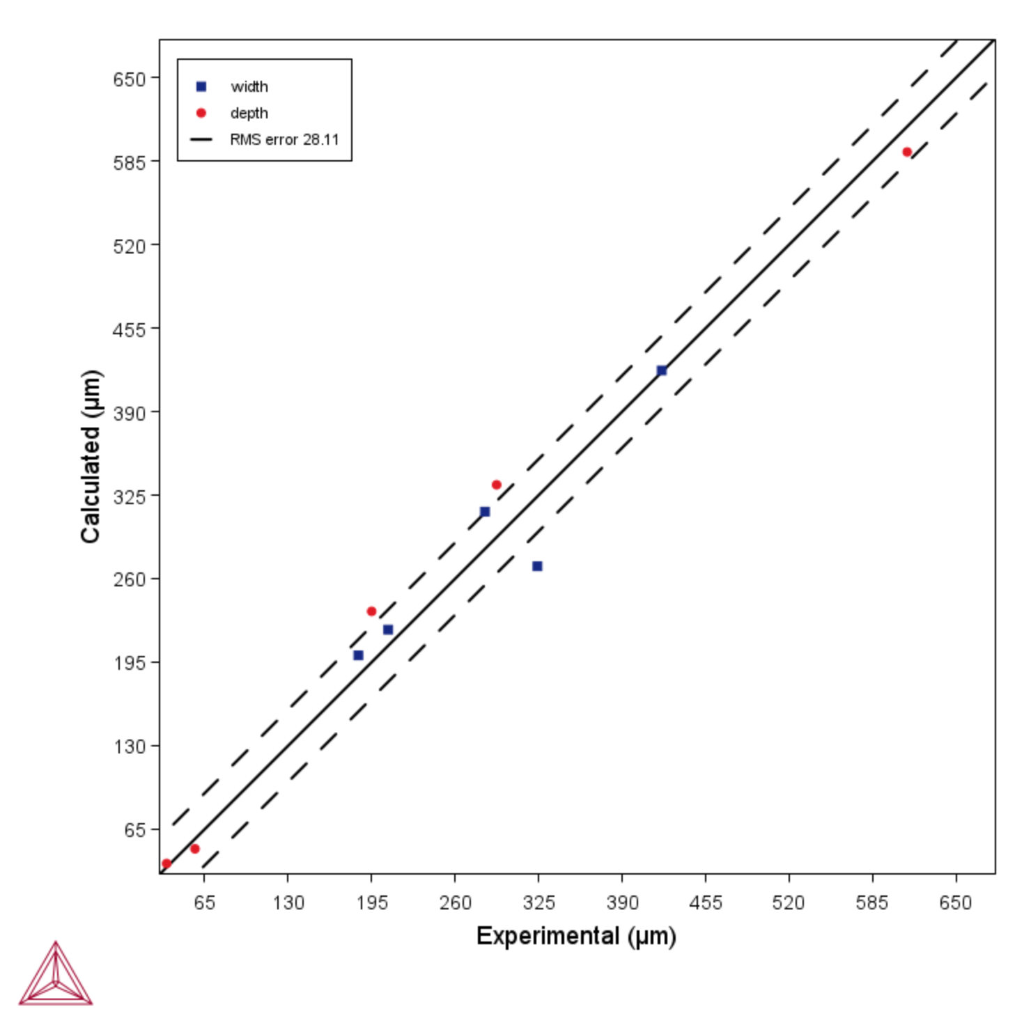
This specific Parity plot is shown by clicking the Parity Plot node in the Project window. Then you can see on the Visualizations window it is in the tab of the same name. The settings are located on the Configuration window on the Batch tab.
The plot compares experimental and calculated melt pool width and depth for all experiments. The experiments are single tracks on bare plate SS316L with varied power and scan speed using a Core-ring heat source.
Figure 1: Parity plot comparing experimental and calculated melt pool width and depth for all the experiments when using a Core-ring heat source. The Root Mean Square (RMS) error can also be seen as a dashed line.
3D Plots
The specific 3D Plot that is highlighted in this section is shown by clicking the 3D Plot node in the Project window. Then on the Visualizations window on the tab of the same name, you can use various toolbar buttons to navigate and experiment with the views, for example:
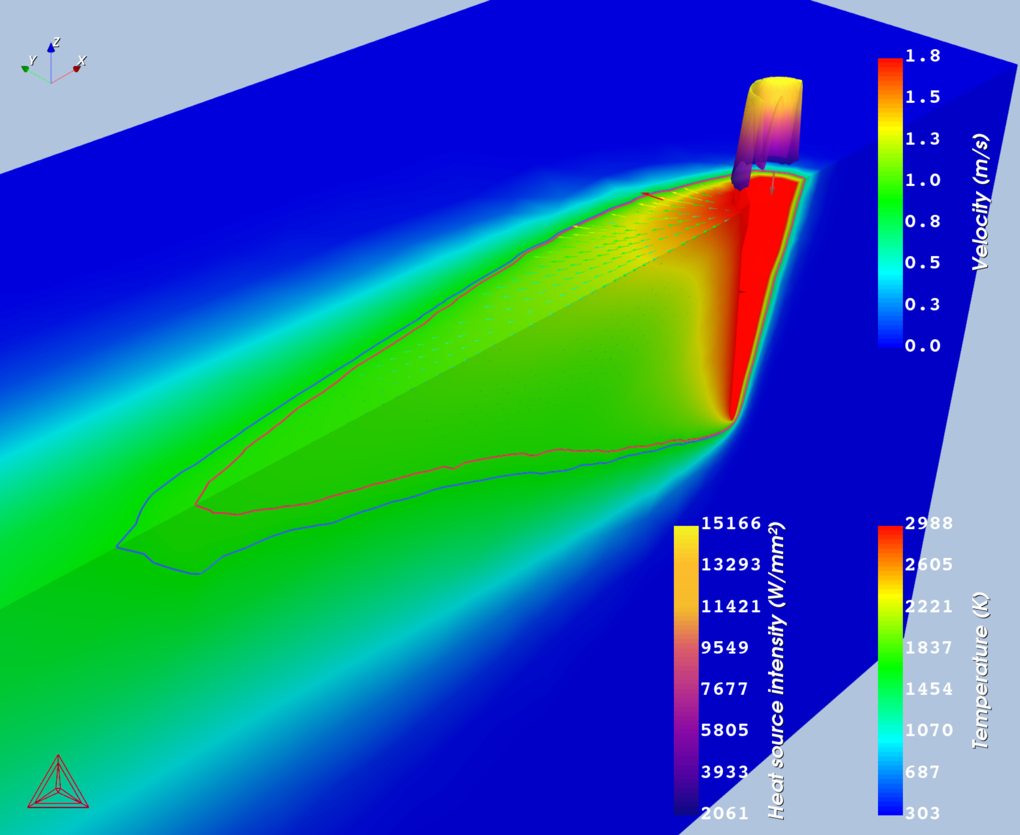
In Figure 2, and using a combination of the Plot Renderer Configuration window settings on the 3D Plot tab and the Visualizations window, different zoom levels and adjusting the Glyph scale factor setting helps to clearly show the melt pool and velocity vectors.
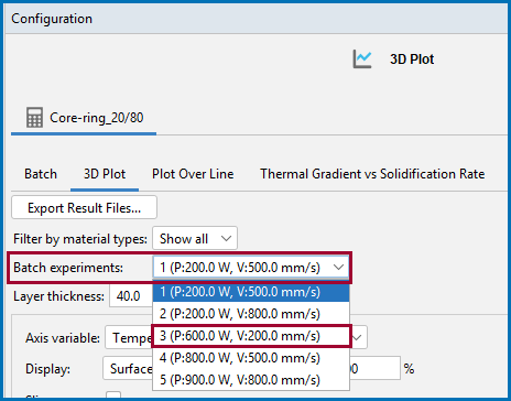
Further, the plot on the left is displayed by choosing the applicable Batch experiments results from the list (P=200 W, V=500 mm/s) and this set of experiments undergoes melting in conduction mode. Then the plot on the right is displayed by choosing the applicable Batch experiments results (P=600 W, V=200 mm/s) and that one forms a keyhole.
|
|
Figure 2: A comparison of the melt pools for two different processing conditions: Red and blue isocontours show liquidus and solidus temperatures, respectively. See the text for details.
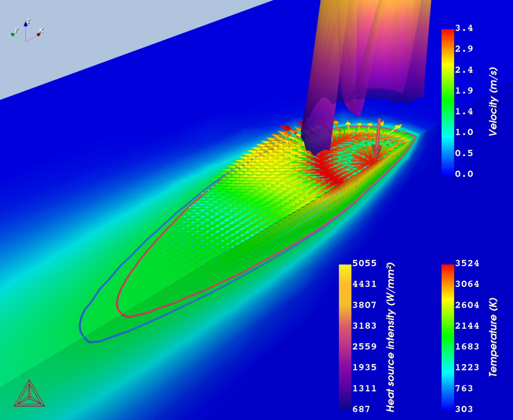
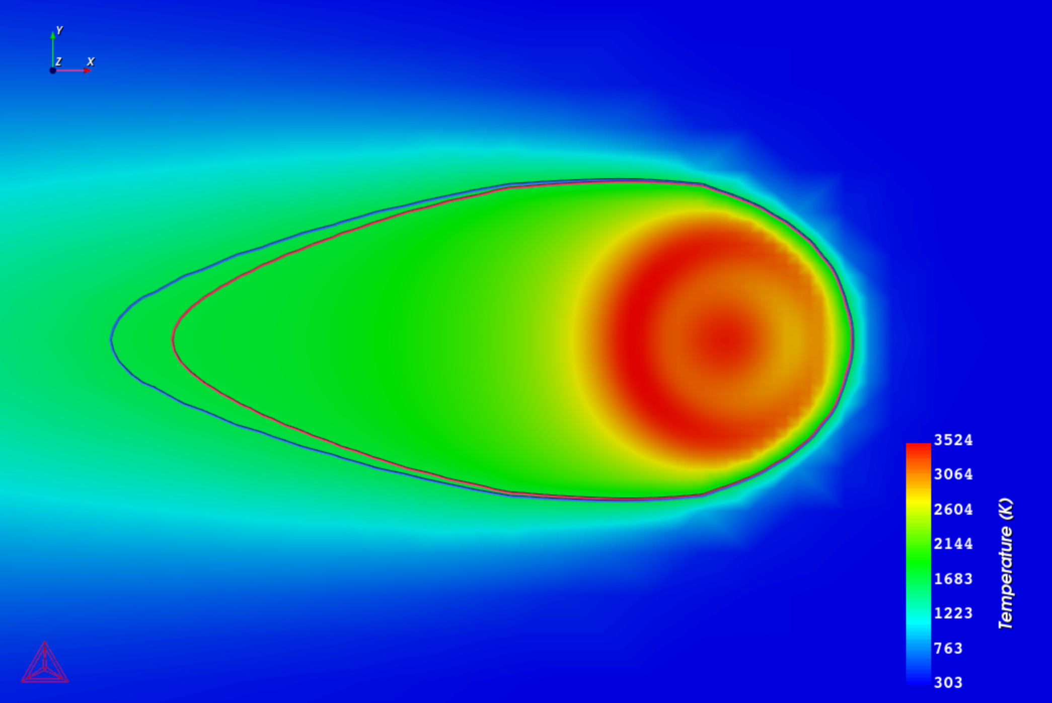
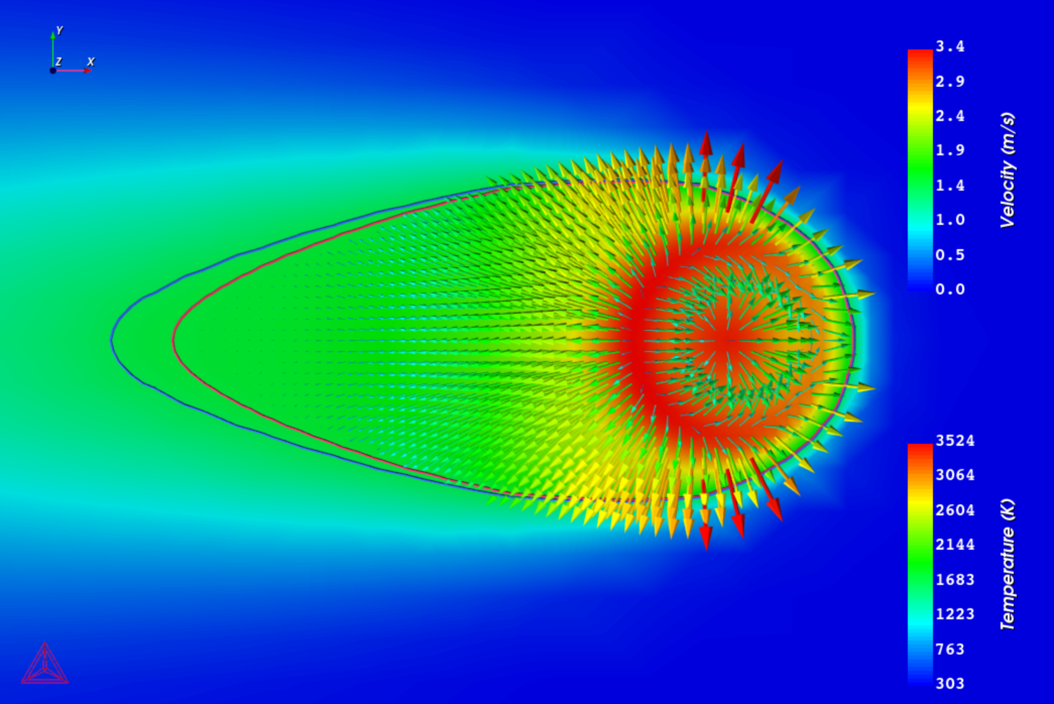
In Figure 3 you can click the  Set View button plus
  Mirror Geometry button to obtain this top view of a Surface colormap.
In general, you can play around with the 3D Plot Configuration window settings. For example, for the right-hand side figure, you can view the Flow velocity field with different Display types such as an Arrow (shown).
|
|
Figure 3: Top view (XY) of the surface colormap showing (left) temperature distribution due to the 20/80 Core-ring beam shape, and (right) velocity field caused by the distinctive temperature profile, resulting in widening of the melt pool. P=200 W, V=500 mm/s. Red and blue isocontours show liquidus and solidus temperatures, respectively.
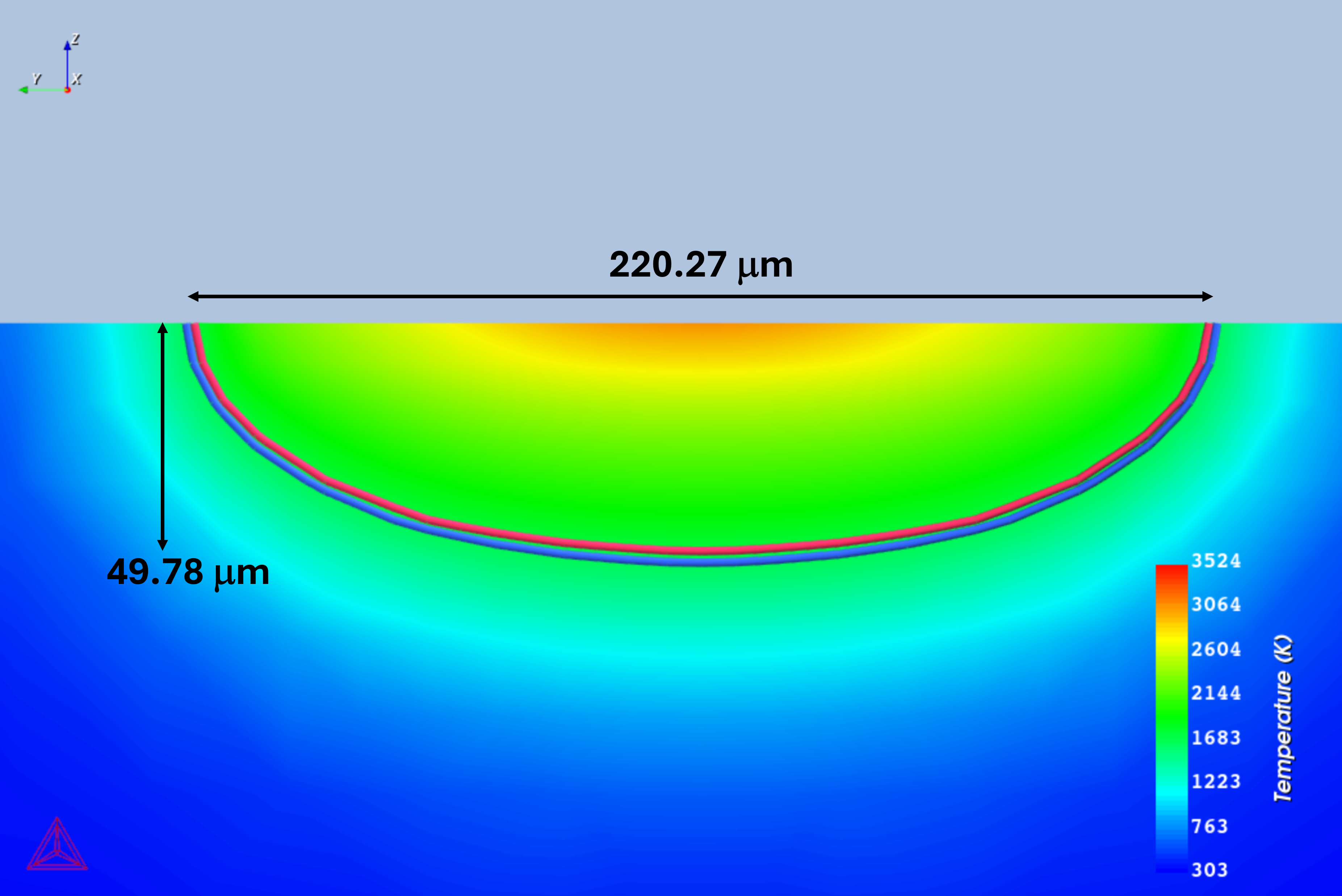
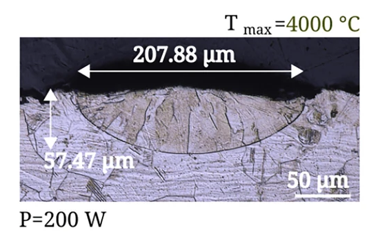
In Figure 4, this cross-section compares the melt pool shape and size for Batch experiment 1 (P=200 W, V=500 mm/s) to the experimental results as shown in Figure 9 in the paper by [2024Hol].
|
|
Figure 4: A cross-section comparing melt pool shape and size for P=200 W, V=500 mm/s from (left) simulation and (right) experiments [2024Hol-Fig9]. Red and blue isocontours in the simulation result show liquidus and solidus temperatures, respectively.
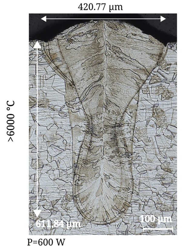
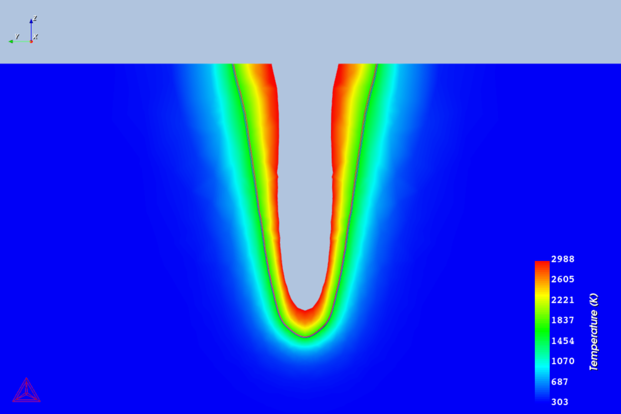
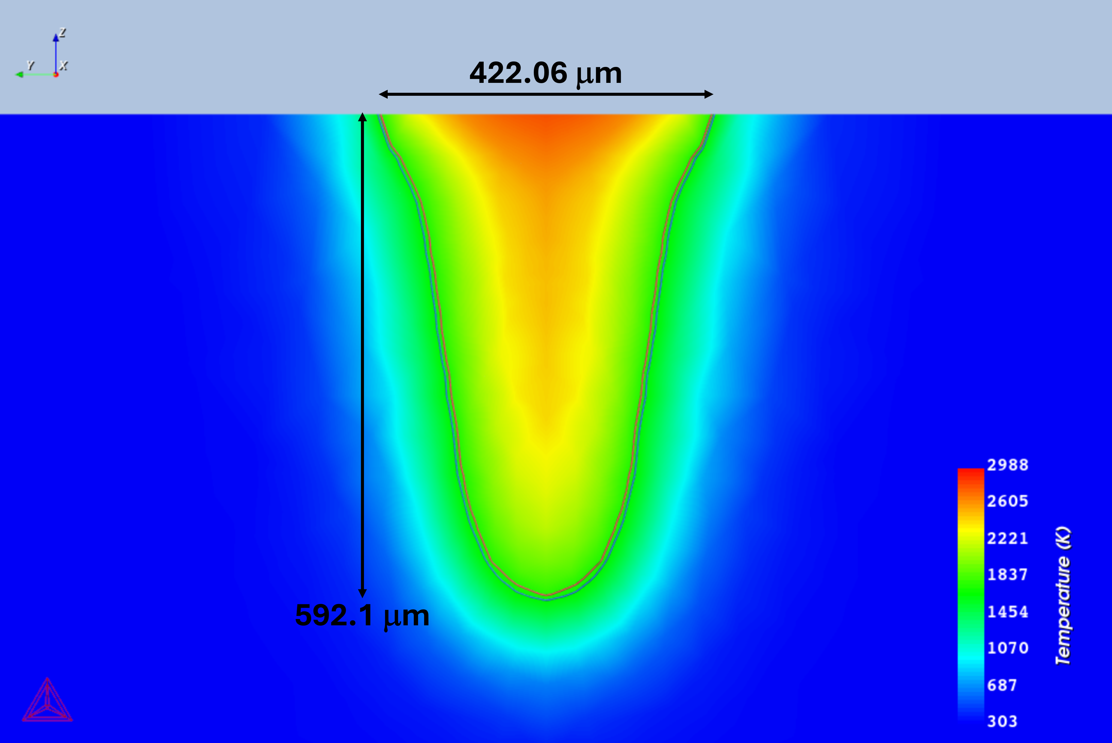
In Figure 5, the formation of the meltpool is shown on the left and compared to a cross-section that is taken from Batch experiment 3 (P=600 W, V=200 mm/s) to show the formation of a keyhole and the maximum melt pool size, where you can also see the widening of the melt pool due to fluid flow. Compare this to Figure 6, which are the experimental results as shown in Figure 9 in the paper by [2024Hol].
|
|
Figure 5: Cross-sections at different locations along the scanning direction showing (left) formation of keyhole and (right) maximum melt pool dimensions for P=600 W, V=200 mm/s. See the text for more.
Figure 6: Cross-section showing the experimental melt track for the same processing conditions shown in Figure 5. From [2024Hol-Fig9].
Other Resources
Read more about the Additive Manufacturing (AM) Module on our website including the details about database compatibility or to watch an introductory webinar. You can also use the Getting Started Guide to learn about the key features available.
Many of our Graphical Mode examples have video tutorials, which you can access in a variety of ways. When in Thermo‑Calc, from the menu select Help → Video Tutorials, or from the main My Project window, click Video Tutorials. Alternately, you can go to the website or our YouTube channel.
References
[2021Grü] J. Grünewald, F. Gehringer, M. Schmöller, K. Wudy, Influence of Ring-Shaped Beam Profiles on Process Stability and Productivity in Laser-Based Powder Bed Fusion of AISI 316L. Metals (Basel). 11, 1989 (2021).
[2023Bi] J. Bi, L. Wu, S. Li, Z. Yang, X. Jia, M. D. Starostenkov, G. Dong, Beam shaping technology and its application in metal laser additive manufacturing: A review. J. Mater. Res. Technol. 26, 4606–4628 (2023).
[2024Hol] V. Holla, J. Grünewald, P. Kopp, P. M. Praegla, C. Meier, K. Wudy, S. Kollmannsberger, Validity of Thermal Simulation Models for Different Laser Beam Shapes in Bead-on-Plate Melting. Integr. Mater. Manuf. Innov. 13, 969–985 (2024).
[2024Hol-Fig9]: V. Holla et. al, Validity of Thermal Simulation Models for Different Laser Beam Shapes in Bead-on-Plate Melting. Integr. Mater. Manuf. Innov. 13, 969–985 (2024). Creative Commons Attribution 4.0 International License, Figure 9, accessed May 2025, cropped individual images from source. https://link.springer.com/article/10.1007/s40192-024-00382-2/figures/9
