AM_14: Using the Top-hat Beam Shape
This Steady-state example demonstrates the use of Top-hat Heat Source model in the AM Module with Batch calculations.
The processing parameters (power and speed) and other processing conditions such as the layer thickness are taken from Sow et al. [2020Sow]. The example also compares the predicted melt pool dimensions with the experimental data.
For TC-Python users, there is an example using Top-hat: pyex_AM_10_TopHat_BeamShape.py.
There is a companion example in Graphical Mode using Core-ring: AM_13: Using the Core-ring Beam Shape.
- Folder: Additive Manufacturing
- File name: AM_14_TopHat_BeamShape.tcu
This example requires an Additive Manufacturing (AM) Module license.
Background
The primary benefit of the Top-hat heat source beam shape, in comparison to the Gaussian beam shape, is uniform energy distribution across the beam spot, leading to even heating of the material surface. With lower peak intensity as compared to the Gaussian beam, a Top-hat beam also allows the use of larger beam size that not only increases productivity but also reduces vapor-induced instabilities [2020Sow]. The inclusion of Top-hat heat source model in the AM Module, together with the keyhole model, allows you to predict the temperature evolution and melt pool shape along with the transition from conduction mode to keyhole mode for a Top-hat heat source. The example uses experimental data taken from the literature [2020Sow] and demonstrates the use of Top-hat heat source with a rather large beam size for single track experiments on an IN625 alloy.
Material Properties
- IN625: Ni-21.5Cr-5.0Fe-0.5Si-0.5Mn-9.0Mo-0.4Ti-1.0Co-1.8Nb-1.8Ta-0.4Al Mass percent
- Database: TCNI12 and with solute trapping and interface scattering = 1e-07.
- The material properties are precalculated, and stored as a built-in material library with the Additive Manufacturing (AM) Module.
AM Calculator Configuration Settings
This example contains one AM Calculator, which is renamed to Top-hat. On the Configuration window, Conditions tab, this Steady-state calculation is configured with the Top-hat Heat Source with the Keyhole model.
Fluid flow is not used in this example (the Fluid flow including Marangoni effect checkbox is not selected). Although fluid flow plays a crucial role in determining the shape and size of the melt pool, in this case it was found that it overestimates the melt pool width for most cases when fluid flow is included.
In the Geometry section, the Height of the base plate is set to 3.0 mm and in the Scanning Strategy section the Layer thickness is changed to 50.0 μm.
In the Heat Source section, the Beam radius is set to 450 μm.
In the [2020Sow] paper, it is mentioned that the beam diameter for the top-hat distribution is 500 μm. However, in Figure 2 of this paper, where intensity is plotted against the distance for the top-hat beam, the actual diameter looks much larger than that. In order to match the intensity distribution, the beam radius is therefore set to 450 μm.
Also in the Heat Source section, the Absorptivity is set to Calculated with a prefactor of 1.0 and in the keyhole model, Beam quality factor M2 is kept as 1.0.
The Batch Calculation Type is used to set up all the conditions from the experiments in a single calculation. In the Batch Experiment Data section, the experimental Power and scan Speed as well as the measured melt pool Width (Exp width) and Depth (Exp. depth) were collected in a CSV file and imported into the software. This data is then saved in the project file.
Data with the error bars is also read and stored in the project file, that is later used to plot error bars together with the experimental values of melt pool width and depth.
In the Batch Experiment Data table, the Power is always 1000 W and the scan Speed ranges between 25 mm/s to 500 mm/s.
AM Calculator Conditions Settings and AM Calculator Heat Source Settings
Visualizations
Open the example project file to review the node setup on the Project window and the associated settings on the Configuration window for each node. For some types of projects, you can also adjust settings on the Plot Renderer Configuration window to preview results before performing the simulation. Click Perform Tree to generate plots and tables to see the results on the Visualizations window.
When you run (Perform) this example, it takes a few minutes for the calculations to complete.
For more information also see Working with AM Visualizations.
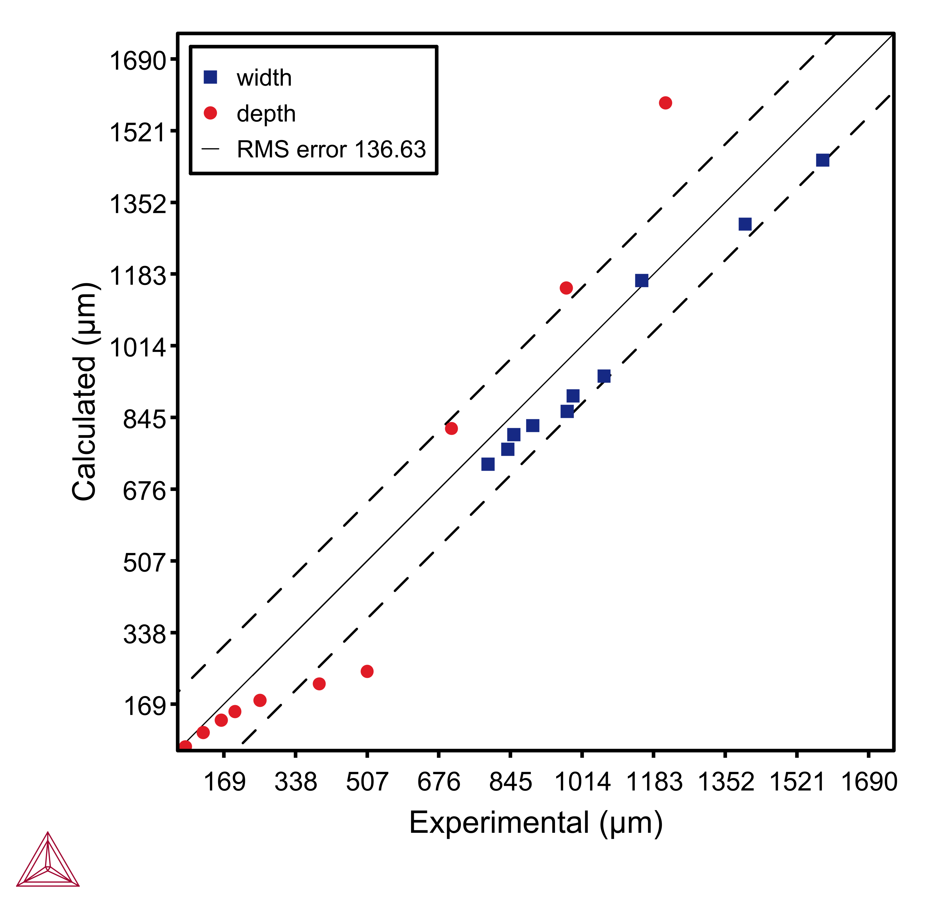
Parity Plot
This specific Parity plot is shown by clicking the Parity Plot node in the Project window. Then you can see on the Visualizations window it is in the tab of the same name. The settings are located on the Configuration window on the Batch tab.
The plot compares experimental and calculated melt pool width and depth. It can be seen that the calculated melt pool width shows a fairly good agreement with the measured values. A mixed trend is however, seen for the melt pool depth. For lower energy densities, the calculated and measured melt pool depth matches quite well, however it starts to deviate once the melting appears to happen in the keyhole mode in the experiments, while it is still in the conduction mode in the calculations. For the last three points, where the calculations also predict a keyhole mode, the melt pool depth matches quite well with the measured value, except for the very last point where it is somehow overpredicted. The difference in depth could be attributed to the uncertainty in the actual beam size of the top-hat beam.
Figure 1: Parity plot comparing experimental and calculated melt pool width and depth for all the experiments. The experiments are single tracks on IN625 with constant power and varied scan speed using the Top-hat heat source. The Root Mean Square (RMS) error can also be seen as a dashed line.
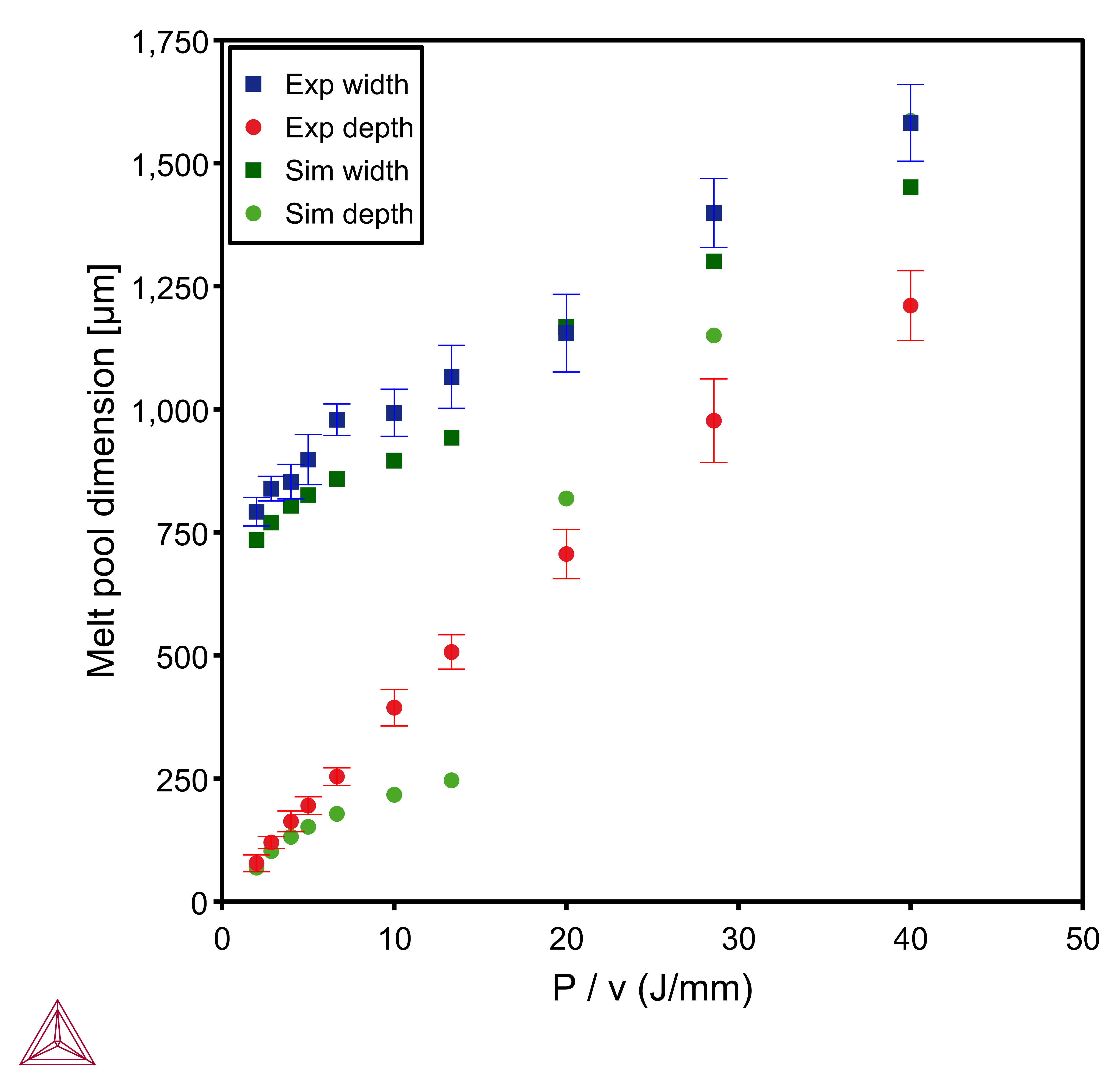
Melt Pool Dimensions
This Melt Pool vs Energy Density plot is shown by clicking the Melt Pool Dimensions node in the Project window. Then you can see on the Visualizations window it is in the tab of the same name. The settings are located on the Configuration window on the Batch tab.
The plot shows a comparison of the experimental and calculated melt pool width and depth, where the error bars are also plotted with the measured data. Rather large error bars, especially for the higher energy density cases, show that the overall trend for the calculated values of melt pool width and depth is in good agreement with the measured values. Some improvements are however needed for the low energy density cases where a huge deviation is found between the calculated and measured values.
Figure 2: A comparison of the experimental and calculated melt pool width and depth for all the experiments. The error bars on the experimental data are also shown.
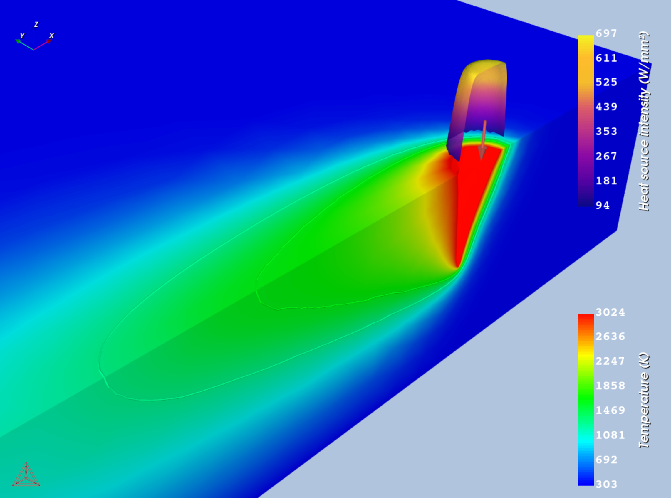
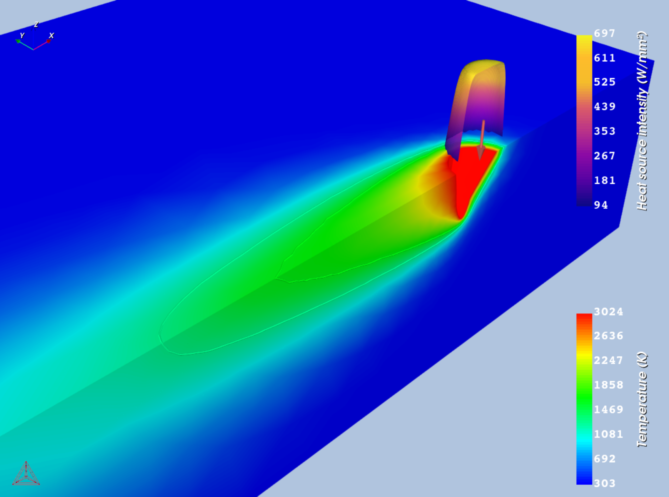
3D Plots
|
|
|
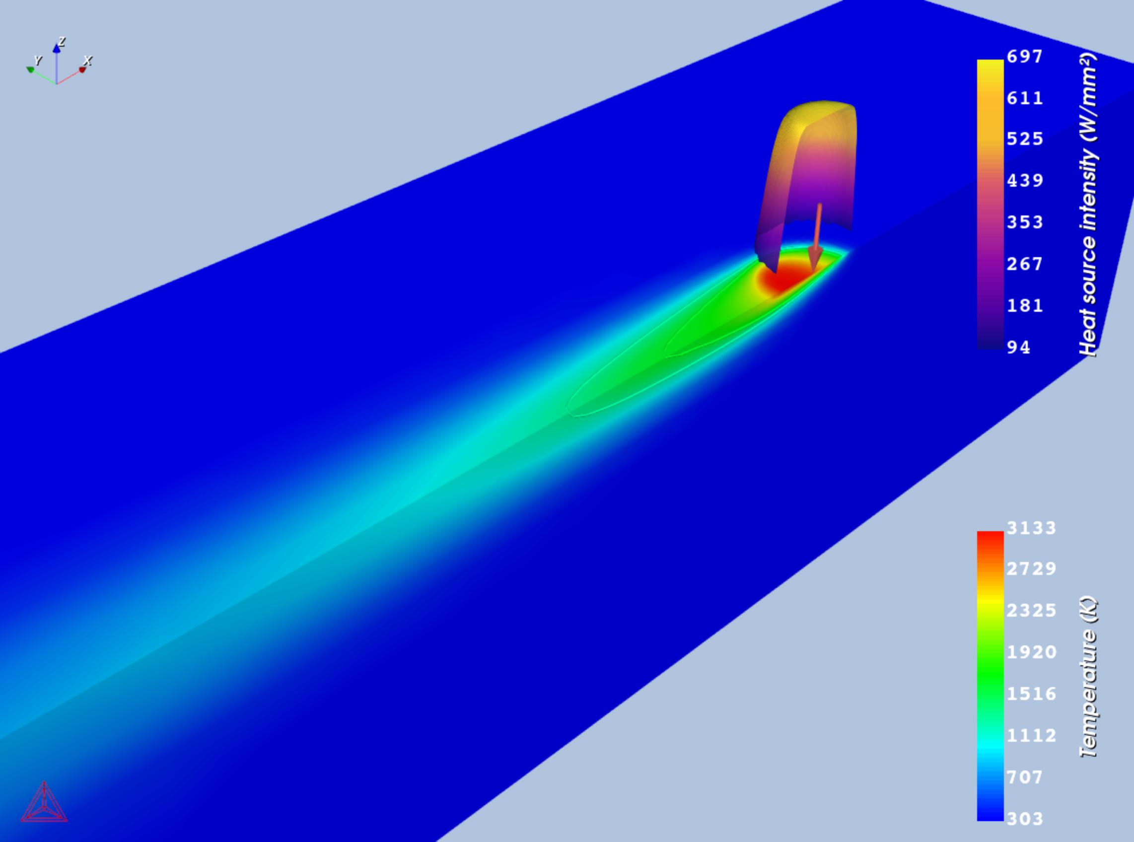
Figure 3: A comparison of the temperature distribution for three different processing conditions: (top-left) P=1000 W, V=25 mm/s, (top-right) P=1000 W, V=50 mm/s, both of which form keyhole during melting and (bottom-left) P=1000 W, V=250 mm/s that undergoes melting in conduction mode.
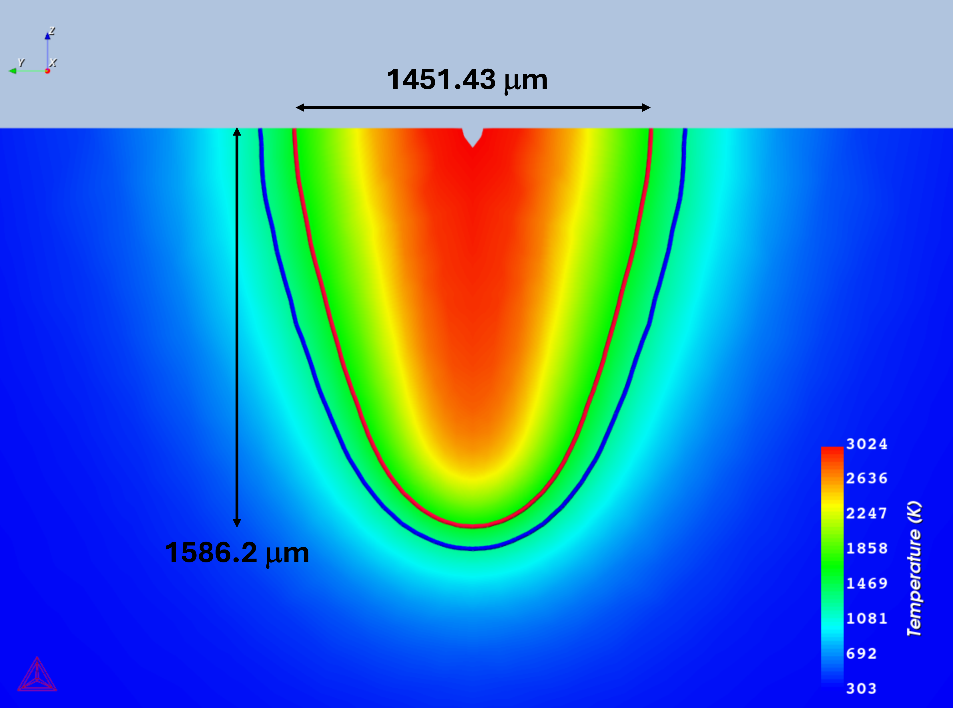
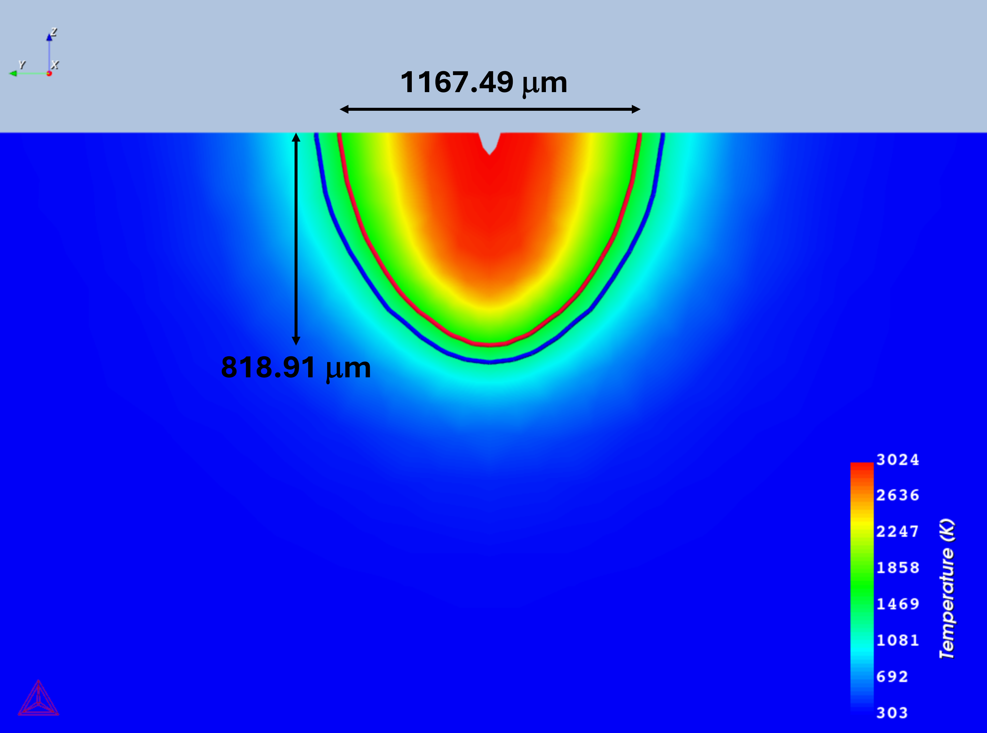
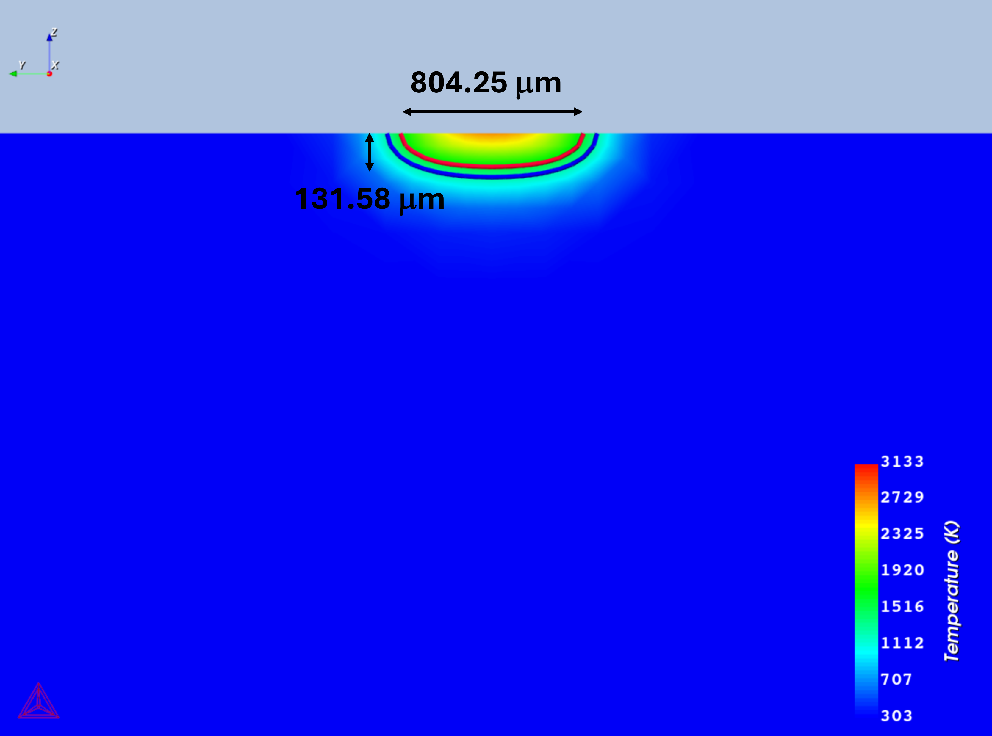
For the comparisons in Figure 4, all cross-sections are taken where the melt pools attain maximum width and depth. Red and blue isocontours show liquidus and solidus temperatures, respectively.
|
|
|
Figure 4: Cross-sections comparing melt pool shape and size for (top-left) P=1000 W, V=25 mm/s, (top-right) P=1000 W, V=50 mm/s and (bottom-left) P=1000 W, V=250 mm/s.
Other Resources
Read more about the Additive Manufacturing (AM) Module on our website including the details about database compatibility or to watch an introductory webinar. You can also use the Getting Started Guide to learn about the key features available.
Many of our Graphical Mode examples have video tutorials, which you can access in a variety of ways. When in Thermo‑Calc, from the menu select Help → Video Tutorials, or from the main My Project window, click Video Tutorials. Alternately, you can go to the website or our YouTube channel.
Reference
[2020Sow] M. C. Sow, T. De Terris, O. Castelnau, Z. Hamouche, F. Coste, R. Fabbro, P. Peyre, Influence of beam diameter on Laser Powder Bed Fusion (L-PBF) process. Addit. Manuf. 36, 101532 (2020).
