AM_08a: Grid Calculation for a Ti64 Alloy
This example shows the use of the AM Calculator with a Steady-state mode and Grid Calculation Type where it compares the calculated and measured printability map. Printability maps are also known as process maps. The experiments are from Dilip et. al [2017Dil] where they performed single track experiments with the alloy Ti64 at different power and scan speeds. They also printed cubes and performed measurements of the porosity amounts for each experimental condition.
The use of different Plot types in this example include a Printability map and a 3D plot with surface colormap.
This example is part of a set using a Steady-state simulation with a Gaussian heat source, plus the Keyhole model including Fluid flow. These examples collectively show the use of Batch and Grid calculation types plus various plot types such as Printability maps, Parity plots, and Melt pool vs energy density. The examples are numbered AM_07 to AM_09b.
- Folder: Additive Manufacturing
- File name:
AM_08a_Printability_Map_Ti64.tcu
This example requires an Additive Manufacturing (AM) Module license.
Configuration and Calculation Set Up
Below highlights some of the settings for this example to compare with experimental data of Ti64.
This example builds on the previous one (AM_07) and it is recommended to review this and to open the example file to locate and follow along for the settings described here and found on the Configuration window.
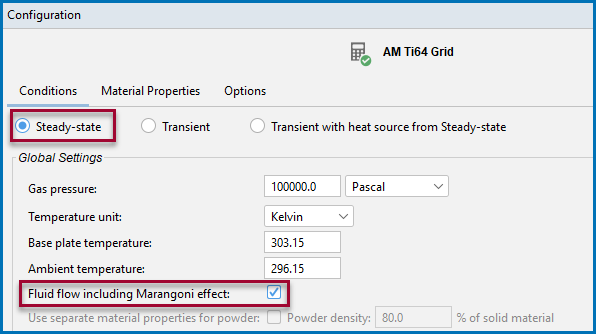
The Steady-state calculation includes Fluid flow.
The Heat Source is set to Gaussian and uses the Keyhole model. The printers in the experiments had a beam diameter of 100 μm so the Gaussian Beam radius is set to 50 μm. The Absorptivity is set to Calculated.

The Ti6Al4V from project file material is selected from the Material Properties library. The material properties are precalculated and stored as a built-in material Library.

The Grid Calculation Type is used to cover all the conditions from the experiments in a single calculation. The Power ranges between 50‑200 W and the Scanning speed ranges between 500‑1200 mm/s.

Visualizations
Open the example project file to review the node setup on the Project window and the associated settings on the Configuration window for each node. For some types of projects, you can also adjust settings on the Plot Renderer Configuration window to preview results before performing the simulation. Click Perform Tree to generate plots and tables to see the results on the Visualizations window.
When you run (Perform) this example, it can take around two hours to complete the calculations.
There is a wide variety of information shown both in the Visualizations and Plot Renderer Configuration windows that can be viewed during configuration and after performing the calculation(s). Not all views, such as the Geometry or previews, nor all additional output (i.e. plots) are shown in this section and it is recommended that you open and run the example to review all available options and results.
Plot Renderer Configuration Window
The combined results from the Grid calculation can be viewed under the matching Grid tab on the Plot Renderer Configuration window where it is set to use the Printability map plot type. In this example, the Plot Renderer node is renamed to Printability map in the Project window.

The experimental value of 30 μm powder thickness (Layer thickness) and 100 μm for the Hatch distance seems to be too big to produce dense builds according to this lack of fusion criteria. Full density can then in principle only be achieved by melting the regions between tracks by shifting the layers printed on top so the full depth of the melt pool covers unmelted regions.
 had to be reduced to from 1.0 to 0.45 in order to not extend the lack of fusion region to experimental regions where little porosity was found.")
Printability Map and 3D Plot
There is a video tutorial about the Printability Map on our website and on our YouTube channel. It is also included in the Additive Manufacturing Module YouTube playlist.
 and lack-of-fusion porosity to the lower right.")
Figure 1: The calculated printability map for Ti64 showing the regions for keyholing porosity (upper left) and lack of fusion porosity to the lower right. The labels show the measured amount of porosity. Labels in red show regions with severe amounts of porosity and labels in black/green show regions with little or no defects.

Figure 2: 3D plot showing a keyhole for the simulation that uses power 200 W and scan speed 1200 mm/s.
Reference
[2017Dil] J. J. S. Dilip, S. Zhang, C. Teng, K. Zeng, C. Robinson, D. Pal, B. Stucker, Influence of processing parameters on the evolution of melt pool, porosity, and microstructures in Ti-6Al-4V alloy parts fabricated by selective laser melting. Prog. Addit. Manuf. 2, 157–167 (2017).
Other Resources
Read more about the Additive Manufacturing (AM) Module on our website including the details about database compatibility or to watch an introductory webinar. You can also use the Getting Started Guide to learn about the key features available.